
Средняя квадратичная ошибка.
При ответственных
измерениях, когда необходимо знать
надежность полученных результатов,
используется средняя квадратичная
ошибка (или
стандартное отклонение), которая
определяется формулой
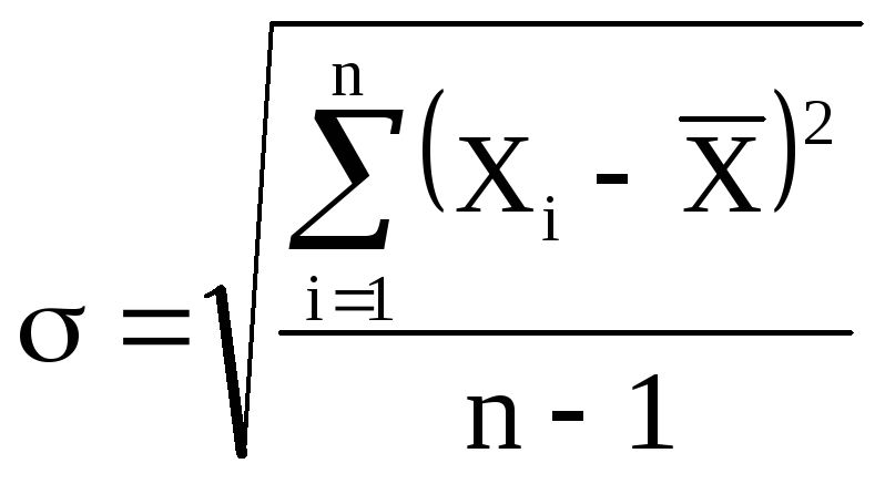
(5)
Величина
характеризует отклонение отдельного
единичного измерения от истинного
значения.
Если мы вычислили
по n
измерениям среднее значение
![]()
по формуле (2), то это значение будет
более точным, то есть будет меньше
отличаться от истинного, чем каждое
отдельное измерение. Средняя квадратичная
ошибка среднего значения
![]()
равна
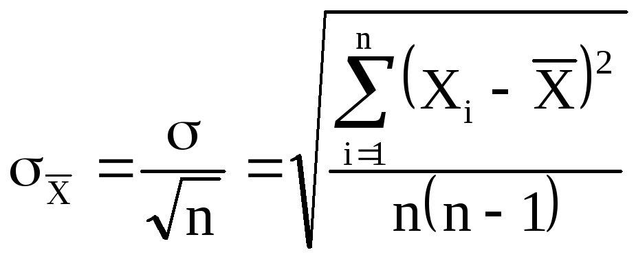
(6)
где — среднеквадратичная
ошибка каждого отдельного измерения,
n
– число измерений.
Таким образом,
увеличивая число опытов, можно уменьшить
случайную ошибку в величине среднего
значения.
В настоящее время
результаты научных и технических
измерений принято представлять в виде
![]()
(7)
Как показывает
теория, при такой записи мы знаем
надежность полученного результата, а
именно, что истинная величина Х с
вероятностью 68% отличается от
![]()
не более, чем на
![]() .
.
При использовании
же средней арифметической (абсолютной)
ошибки (формула 2) о надежности результата
ничего сказать нельзя. Некоторое
представление о точности проведенных
измерений в этом случае дает относительная
ошибка (формула 4).
При выполнении
лабораторных работ студенты могут
использовать как среднюю абсолютную
ошибку, так и среднюю квадратичную.
Какую из них применять указывается
непосредственно в каждой конкретной
работе (или указывается преподавателем).
Обычно если число
измерений не превышает 3 – 5, то
можно использовать среднюю абсолютную
ошибку. Если число измерений порядка
10 и более, то следует использовать более
корректную оценку с помощью средней
квадратичной ошибки среднего (формулы
5 и 6).
Учет систематических ошибок.
Увеличением числа
измерений можно уменьшить только
случайные ошибки опыта, но не
систематические.
Максимальное
значение систематической ошибки обычно
указывается на приборе или в его паспорте.
Для измерений с помощью обычной
металлической линейки систематическая
ошибка составляет не менее 0,5 мм; для
измерений штангенциркулем –
0,1 – 0,05 мм;
микрометром – 0,01 мм.
Часто в качестве
систематической ошибки берется половина
цены деления прибора.
На шкалах
электроизмерительных приборов указывается
класс точности. Зная класс точности К,
можно вычислить систематическую ошибку
прибора ∆Х по формуле
![]()
где К – класс
точности прибора, Хпр – предельное
значение величины, которое может быть
измерено по шкале прибора.
Так, амперметр
класса 0,5 со шкалой до 5А измеряет ток с
ошибкой не более
![]()
Погрешность
цифрового прибора равна единице
наименьшего индицируемого разряда.
Среднее значение
полной погрешности складывается из
случайной и систематической
погрешностей.
![]()
Ответ с учетом
систематических и случайных ошибок
записывается в виде
![]()
Погрешности косвенных измерений
В физических
экспериментах чаще бывает так, что
искомая физическая величина сама на
опыте измерена быть не может, а является
функцией других величин, измеряемых
непосредственно. Например, чтобы
определить объём цилиндра, надо измерить
диаметр D и высоту h, а затем вычислить
объем по формуле
![]()
Величины D и h будут измерены с
некоторой ошибкой. Следовательно,
вычисленная величина V
получится также с некоторой ошибкой.
Надо уметь выражать погрешность
вычисленной величины через погрешности
измеренных величин.
Как и при прямых
измерениях можно вычислять среднюю
абсолютную (среднюю арифметическую)
ошибку или среднюю квадратичную ошибку.
Общие правила
вычисления ошибок для обоих случаев
выводятся с помощью дифференциального
исчисления.
Пусть искомая
величина φ является функцией нескольких
переменных Х,
У, Z…
φ(Х,
У, Z…).
Путем прямых
измерений мы можем найти величины
![]() ,
,
а также оценить их средние абсолютные
ошибки
![]() …
…
или средние квадратичные ошибки Х,
У,
Z…
Тогда средняя
арифметическая погрешность
вычисляется по формуле
![]()
где
![]() — частные
— частные
производные от φ по
Х, У, Z. Они
вычисляются для средних значений
![]() …
…
Средняя квадратичная
погрешность вычисляется по формуле
![]()
Пример.
Выведем формулы погрешности для
вычисления объёма цилиндра.
а) Средняя
арифметическая погрешность.
Величины
D и h
измеряются соответственно с ошибкой
D
и h.
Погрешность
величины объёма будет равна
![]()
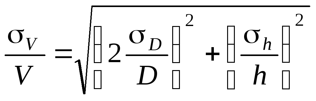
б) Средняя
квадратичная погрешность.
Величины
D и h
измеряются соответственно с ошибкой
D,
h.
Погрешность
величины объёма будет равна
![]()
Если формула
представляет выражение удобное для
логарифмирования (то есть произведение,
дробь, степень), то удобнее вначале
вычислять относительную погрешность.
Для этого (в случае средней арифметической
погрешности) надо проделать следующее.
1. Прологарифмировать
выражение.
2. Продифференцировать
его.
3. Объединить
все члены с одинаковым дифференциалом
и вынести его за скобки.
4. Взять выражение
перед различными дифференциалами по
модулю.
5. Заменить
значки дифференциалов d
на значки абсолютной погрешности .
В итоге получится
формула для относительной погрешности
![]()
Затем,
зная ,
можно вычислить абсолютную погрешность
=
Пример.
![]()
![]()
![]()
![]()
Аналогично можно
записать относительную среднюю
квадратичную погрешность
Правила
представления результатов измерения
следующие:
-
погрешность должна
округляться до одной значащей цифры:
правильно = 0,04,
неправильно —
= 0,0382;
-
последняя значащая
цифра результата должна быть того же
порядка величины, что и погрешность:
правильно
= 9,830,03,
неправильно —
= 9,8260,03;
-
если результат
имеет очень большую или очень малую
величину, необходимо использовать
показательную форму записи — одну и ту
же для результата и его погрешности,
причем запятая десятичной дроби должна
следовать за первой значащей цифрой
результата:
правильно —
= (5,270,03)10-5,
неправильно —
= 0,00005270,0000003,
= 5,2710-50,0000003,
=
= 0,0000527310-7,
= (5273)10-7,
= (0,5270,003)
10-4.
-
Если результат
имеет размерность, ее необходимо
указать:
правильно – g=(9,820,02)
м/c2,
неправильно – g=(9,820,02).
Соседние файлы в папке Методички физика
- #
02.04.2015275.46 Кб40оформление заготовки и отчета.ppt
- #
From Wikipedia, the free encyclopedia
In statistics, the mean squared error (MSE)[1] or mean squared deviation (MSD) of an estimator (of a procedure for estimating an unobserved quantity) measures the average of the squares of the errors—that is, the average squared difference between the estimated values and the actual value. MSE is a risk function, corresponding to the expected value of the squared error loss.[2] The fact that MSE is almost always strictly positive (and not zero) is because of randomness or because the estimator does not account for information that could produce a more accurate estimate.[3] In machine learning, specifically empirical risk minimization, MSE may refer to the empirical risk (the average loss on an observed data set), as an estimate of the true MSE (the true risk: the average loss on the actual population distribution).
The MSE is a measure of the quality of an estimator. As it is derived from the square of Euclidean distance, it is always a positive value that decreases as the error approaches zero.
The MSE is the second moment (about the origin) of the error, and thus incorporates both the variance of the estimator (how widely spread the estimates are from one data sample to another) and its bias (how far off the average estimated value is from the true value).[citation needed] For an unbiased estimator, the MSE is the variance of the estimator. Like the variance, MSE has the same units of measurement as the square of the quantity being estimated. In an analogy to standard deviation, taking the square root of MSE yields the root-mean-square error or root-mean-square deviation (RMSE or RMSD), which has the same units as the quantity being estimated; for an unbiased estimator, the RMSE is the square root of the variance, known as the standard error.
Definition and basic properties[edit]
The MSE either assesses the quality of a predictor (i.e., a function mapping arbitrary inputs to a sample of values of some random variable), or of an estimator (i.e., a mathematical function mapping a sample of data to an estimate of a parameter of the population from which the data is sampled). The definition of an MSE differs according to whether one is describing a predictor or an estimator.
Predictor[edit]
If a vector of  predictions is generated from a sample of data points on all variables, and
  is the vector of observed values of the variable being predicted, with
  being the predicted values (e.g. as from a least-squares fit), then the within-sample MSE of the predictor is computed as

In other words, the MSE is the mean  of the squares of the errors
  . This is an easily computable quantity for a particular sample (and hence is sample-dependent).
In matrix notation,

where  is
is  and
and  is the
  column vector.
The MSE can also be computed on q data points that were not used in estimating the model, either because they were held back for this purpose, or because these data have been newly obtained. Within this process, known as statistical learning, the MSE is often called the test MSE,[4] and is computed as

Estimator[edit]
The MSE of an estimator  with respect to an unknown parameter
  is defined as[1]
![{displaystyle operatorname {MSE} ({hat {theta }})=operatorname {E} _{theta }left[({hat {theta }}-theta )^{2}right].}](https://wikimedia.org/api/rest_v1/media/math/render/svg/9a0e1b3bac58f9ba2d2f4ff8b85b2e35a8f4bf78)
This definition depends on the unknown parameter, but the MSE is a priori a property of an estimator. The MSE could be a function of unknown parameters, in which case any estimator of the MSE based on estimates of these parameters would be a function of the data (and thus a random variable). If the estimator is derived as a sample statistic and is used to estimate some population parameter, then the expectation is with respect to the sampling distribution of the sample statistic.
The MSE can be written as the sum of the variance of the estimator and the squared bias of the estimator, providing a useful way to calculate the MSE and implying that in the case of unbiased estimators, the MSE and variance are equivalent.[5]

Proof of variance and bias relationship[edit]
![{displaystyle {begin{aligned}operatorname {MSE} ({hat {theta }})&=operatorname {E} _{theta }left[({hat {theta }}-theta )^{2}right]\&=operatorname {E} _{theta }left[left({hat {theta }}-operatorname {E} _{theta }[{hat {theta }}]+operatorname {E} _{theta }[{hat {theta }}]-theta right)^{2}right]\&=operatorname {E} _{theta }left[left({hat {theta }}-operatorname {E} _{theta }[{hat {theta }}]right)^{2}+2left({hat {theta }}-operatorname {E} _{theta }[{hat {theta }}]right)left(operatorname {E} _{theta }[{hat {theta }}]-theta right)+left(operatorname {E} _{theta }[{hat {theta }}]-theta right)^{2}right]\&=operatorname {E} _{theta }left[left({hat {theta }}-operatorname {E} _{theta }[{hat {theta }}]right)^{2}right]+operatorname {E} _{theta }left[2left({hat {theta }}-operatorname {E} _{theta }[{hat {theta }}]right)left(operatorname {E} _{theta }[{hat {theta }}]-theta right)right]+operatorname {E} _{theta }left[left(operatorname {E} _{theta }[{hat {theta }}]-theta right)^{2}right]\&=operatorname {E} _{theta }left[left({hat {theta }}-operatorname {E} _{theta }[{hat {theta }}]right)^{2}right]+2left(operatorname {E} _{theta }[{hat {theta }}]-theta right)operatorname {E} _{theta }left[{hat {theta }}-operatorname {E} _{theta }[{hat {theta }}]right]+left(operatorname {E} _{theta }[{hat {theta }}]-theta right)^{2}&&operatorname {E} _{theta }[{hat {theta }}]-theta ={text{const.}}\&=operatorname {E} _{theta }left[left({hat {theta }}-operatorname {E} _{theta }[{hat {theta }}]right)^{2}right]+2left(operatorname {E} _{theta }[{hat {theta }}]-theta right)left(operatorname {E} _{theta }[{hat {theta }}]-operatorname {E} _{theta }[{hat {theta }}]right)+left(operatorname {E} _{theta }[{hat {theta }}]-theta right)^{2}&&operatorname {E} _{theta }[{hat {theta }}]={text{const.}}\&=operatorname {E} _{theta }left[left({hat {theta }}-operatorname {E} _{theta }[{hat {theta }}]right)^{2}right]+left(operatorname {E} _{theta }[{hat {theta }}]-theta right)^{2}\&=operatorname {Var} _{theta }({hat {theta }})+operatorname {Bias} _{theta }({hat {theta }},theta )^{2}end{aligned}}}](https://wikimedia.org/api/rest_v1/media/math/render/svg/2ac524a751828f971013e1297a33ca1cc4c38cd6)
An even shorter proof can be achieved using the well-known formula that for a random variable  ,
,  . By substituting with,
  , we have
![{displaystyle {begin{aligned}operatorname {MSE} ({hat {theta }})&=mathbb {E} [({hat {theta }}-theta )^{2}]\&=operatorname {Var} ({hat {theta }}-theta )+(mathbb {E} [{hat {theta }}-theta ])^{2}\&=operatorname {Var} ({hat {theta }})+operatorname {Bias} ^{2}({hat {theta }})end{aligned}}}](https://wikimedia.org/api/rest_v1/media/math/render/svg/864646cf4426e2b62a3caf9460382eec1a77fe4e)
But in real modeling case, MSE could be described as the addition of model variance, model bias, and irreducible uncertainty (see Bias–variance tradeoff). According to the relationship, the MSE of the estimators could be simply used for the efficiency comparison, which includes the information of estimator variance and bias. This is called MSE criterion.
In regression[edit]
In regression analysis, plotting is a more natural way to view the overall trend of the whole data. The mean of the distance from each point to the predicted regression model can be calculated, and shown as the mean squared error. The squaring is critical to reduce the complexity with negative signs. To minimize MSE, the model could be more accurate, which would mean the model is closer to actual data. One example of a linear regression using this method is the least squares method—which evaluates appropriateness of linear regression model to model bivariate dataset,[6] but whose limitation is related to known distribution of the data.
The term mean squared error is sometimes used to refer to the unbiased estimate of error variance: the residual sum of squares divided by the number of degrees of freedom. This definition for a known, computed quantity differs from the above definition for the computed MSE of a predictor, in that a different denominator is used. The denominator is the sample size reduced by the number of model parameters estimated from the same data, (n−p) for p regressors or (n−p−1) if an intercept is used (see errors and residuals in statistics for more details).[7] Although the MSE (as defined in this article) is not an unbiased estimator of the error variance, it is consistent, given the consistency of the predictor.
In regression analysis, «mean squared error», often referred to as mean squared prediction error or «out-of-sample mean squared error», can also refer to the mean value of the squared deviations of the predictions from the true values, over an out-of-sample test space, generated by a model estimated over a particular sample space. This also is a known, computed quantity, and it varies by sample and by out-of-sample test space.
Examples[edit]
Mean[edit]
Suppose we have a random sample of size from a population,  . Suppose the sample units were chosen with replacement. That is, the units are selected one at a time, and previously selected units are still eligible for selection for all draws. The usual estimator for the
  is the sample average

which has an expected value equal to the true mean (so it is unbiased) and a mean squared error of
![{displaystyle operatorname {MSE} left({overline {X}}right)=operatorname {E} left[left({overline {X}}-mu right)^{2}right]=left({frac {sigma }{sqrt {n}}}right)^{2}={frac {sigma ^{2}}{n}}}](https://wikimedia.org/api/rest_v1/media/math/render/svg/b4647a2cc4c8f9a4c90b628faad2dcf80c4aae84)
where  is the population variance.
For a Gaussian distribution, this is the best unbiased estimator (i.e., one with the lowest MSE among all unbiased estimators), but not, say, for a uniform distribution.
Variance[edit]
The usual estimator for the variance is the corrected sample variance:

This is unbiased (its expected value is ), hence also called the unbiased sample variance, and its MSE is[8]

where  is the fourth central moment of the distribution or population, and
  is the excess kurtosis.
However, one can use other estimators for which are proportional to  , and an appropriate choice can always give a lower mean squared error. If we define

then we calculate:
![{displaystyle {begin{aligned}operatorname {MSE} (S_{a}^{2})&=operatorname {E} left[left({frac {n-1}{a}}S_{n-1}^{2}-sigma ^{2}right)^{2}right]\&=operatorname {E} left[{frac {(n-1)^{2}}{a^{2}}}S_{n-1}^{4}-2left({frac {n-1}{a}}S_{n-1}^{2}right)sigma ^{2}+sigma ^{4}right]\&={frac {(n-1)^{2}}{a^{2}}}operatorname {E} left[S_{n-1}^{4}right]-2left({frac {n-1}{a}}right)operatorname {E} left[S_{n-1}^{2}right]sigma ^{2}+sigma ^{4}\&={frac {(n-1)^{2}}{a^{2}}}operatorname {E} left[S_{n-1}^{4}right]-2left({frac {n-1}{a}}right)sigma ^{4}+sigma ^{4}&&operatorname {E} left[S_{n-1}^{2}right]=sigma ^{2}\&={frac {(n-1)^{2}}{a^{2}}}left({frac {gamma _{2}}{n}}+{frac {n+1}{n-1}}right)sigma ^{4}-2left({frac {n-1}{a}}right)sigma ^{4}+sigma ^{4}&&operatorname {E} left[S_{n-1}^{4}right]=operatorname {MSE} (S_{n-1}^{2})+sigma ^{4}\&={frac {n-1}{na^{2}}}left((n-1)gamma _{2}+n^{2}+nright)sigma ^{4}-2left({frac {n-1}{a}}right)sigma ^{4}+sigma ^{4}end{aligned}}}](https://wikimedia.org/api/rest_v1/media/math/render/svg/cf22322412b8454c706d78671e5d94208675a6e0)
This is minimized when

For a Gaussian distribution, where  , this means that the MSE is minimized when dividing the sum by
  . The minimum excess kurtosis is
  ,[a] which is achieved by a Bernoulli distribution with p = 1/2 (a coin flip), and the MSE is minimized for
  Hence regardless of the kurtosis, we get a «better» estimate (in the sense of having a lower MSE) by scaling down the unbiased estimator a little bit; this is a simple example of a shrinkage estimator: one «shrinks» the estimator towards zero (scales down the unbiased estimator).
Further, while the corrected sample variance is the best unbiased estimator (minimum mean squared error among unbiased estimators) of variance for Gaussian distributions, if the distribution is not Gaussian, then even among unbiased estimators, the best unbiased estimator of the variance may not be 
Gaussian distribution[edit]
The following table gives several estimators of the true parameters of the population, μ and σ2, for the Gaussian case.[9]
| True value | Estimator | Mean squared error |
|---|---|---|
 |
= the unbiased estimator of the population mean,  |

|
 |
= the unbiased estimator of the population variance,  |

|
|
= the biased estimator of the population variance,  |

|
|
= the biased estimator of the population variance,  |

|
Interpretation[edit]
An MSE of zero, meaning that the estimator predicts observations of the parameter with perfect accuracy, is ideal (but typically not possible).
Values of MSE may be used for comparative purposes. Two or more statistical models may be compared using their MSEs—as a measure of how well they explain a given set of observations: An unbiased estimator (estimated from a statistical model) with the smallest variance among all unbiased estimators is the best unbiased estimator or MVUE (Minimum-Variance Unbiased Estimator).
Both analysis of variance and linear regression techniques estimate the MSE as part of the analysis and use the estimated MSE to determine the statistical significance of the factors or predictors under study. The goal of experimental design is to construct experiments in such a way that when the observations are analyzed, the MSE is close to zero relative to the magnitude of at least one of the estimated treatment effects.
In one-way analysis of variance, MSE can be calculated by the division of the sum of squared errors and the degree of freedom. Also, the f-value is the ratio of the mean squared treatment and the MSE.
MSE is also used in several stepwise regression techniques as part of the determination as to how many predictors from a candidate set to include in a model for a given set of observations.
Applications[edit]
- Minimizing MSE is a key criterion in selecting estimators: see minimum mean-square error. Among unbiased estimators, minimizing the MSE is equivalent to minimizing the variance, and the estimator that does this is the minimum variance unbiased estimator. However, a biased estimator may have lower MSE; see estimator bias.
- In statistical modelling the MSE can represent the difference between the actual observations and the observation values predicted by the model. In this context, it is used to determine the extent to which the model fits the data as well as whether removing some explanatory variables is possible without significantly harming the model’s predictive ability.
- In forecasting and prediction, the Brier score is a measure of forecast skill based on MSE.
Loss function[edit]
Squared error loss is one of the most widely used loss functions in statistics[citation needed], though its widespread use stems more from mathematical convenience than considerations of actual loss in applications. Carl Friedrich Gauss, who introduced the use of mean squared error, was aware of its arbitrariness and was in agreement with objections to it on these grounds.[3] The mathematical benefits of mean squared error are particularly evident in its use at analyzing the performance of linear regression, as it allows one to partition the variation in a dataset into variation explained by the model and variation explained by randomness.
Criticism[edit]
The use of mean squared error without question has been criticized by the decision theorist James Berger. Mean squared error is the negative of the expected value of one specific utility function, the quadratic utility function, which may not be the appropriate utility function to use under a given set of circumstances. There are, however, some scenarios where mean squared error can serve as a good approximation to a loss function occurring naturally in an application.[10]
Like variance, mean squared error has the disadvantage of heavily weighting outliers.[11] This is a result of the squaring of each term, which effectively weights large errors more heavily than small ones. This property, undesirable in many applications, has led researchers to use alternatives such as the mean absolute error, or those based on the median.
See also[edit]
- Bias–variance tradeoff
- Hodges’ estimator
- James–Stein estimator
- Mean percentage error
- Mean square quantization error
- Mean square weighted deviation
- Mean squared displacement
- Mean squared prediction error
- Minimum mean square error
- Minimum mean squared error estimator
- Overfitting
- Peak signal-to-noise ratio
Notes[edit]
- ^ This can be proved by Jensen’s inequality as follows. The fourth central moment is an upper bound for the square of variance, so that the least value for their ratio is one, therefore, the least value for the excess kurtosis is −2, achieved, for instance, by a Bernoulli with p=1/2.
References[edit]
- ^ a b «Mean Squared Error (MSE)». www.probabilitycourse.com. Retrieved 2020-09-12.
- ^ Bickel, Peter J.; Doksum, Kjell A. (2015). Mathematical Statistics: Basic Ideas and Selected Topics. Vol. I (Second ed.). p. 20.
If we use quadratic loss, our risk function is called the mean squared error (MSE) …
- ^ a b Lehmann, E. L.; Casella, George (1998). Theory of Point Estimation (2nd ed.). New York: Springer. ISBN 978-0-387-98502-2. MR 1639875.
- ^ Gareth, James; Witten, Daniela; Hastie, Trevor; Tibshirani, Rob (2021). An Introduction to Statistical Learning: with Applications in R. Springer. ISBN 978-1071614174.
- ^ Wackerly, Dennis; Mendenhall, William; Scheaffer, Richard L. (2008). Mathematical Statistics with Applications (7 ed.). Belmont, CA, USA: Thomson Higher Education. ISBN 978-0-495-38508-0.
- ^ A modern introduction to probability and statistics : understanding why and how. Dekking, Michel, 1946-. London: Springer. 2005. ISBN 978-1-85233-896-1. OCLC 262680588.
{{cite book}}: CS1 maint: others (link) - ^ Steel, R.G.D, and Torrie, J. H., Principles and Procedures of Statistics with Special Reference to the Biological Sciences., McGraw Hill, 1960, page 288.
- ^ Mood, A.; Graybill, F.; Boes, D. (1974). Introduction to the Theory of Statistics (3rd ed.). McGraw-Hill. p. 229.
- ^ DeGroot, Morris H. (1980). Probability and Statistics (2nd ed.). Addison-Wesley.
- ^ Berger, James O. (1985). «2.4.2 Certain Standard Loss Functions». Statistical Decision Theory and Bayesian Analysis (2nd ed.). New York: Springer-Verlag. p. 60. ISBN 978-0-387-96098-2. MR 0804611.
- ^ Bermejo, Sergio; Cabestany, Joan (2001). «Oriented principal component analysis for large margin classifiers». Neural Networks. 14 (10): 1447–1461. doi:10.1016/S0893-6080(01)00106-X. PMID 11771723.
Средняя квадратичная ошибка.
При ответственных
измерениях, когда необходимо знать
надежность полученных результатов,
используется средняя квадратичная
ошибка (или
стандартное отклонение), которая
определяется формулой
(5)
Величина
характеризует отклонение отдельного
единичного измерения от истинного
значения.
Если мы вычислили
по n
измерениям среднее значение
![]()
по формуле (2), то это значение будет
более точным, то есть будет меньше
отличаться от истинного, чем каждое
отдельное измерение. Средняя квадратичная
ошибка среднего значения
![]()
равна
(6)
где — среднеквадратичная
ошибка каждого отдельного измерения,
n
– число измерений.
Таким образом,
увеличивая число опытов, можно уменьшить
случайную ошибку в величине среднего
значения.
В настоящее время
результаты научных и технических
измерений принято представлять в виде
![]()
(7)
Как показывает
теория, при такой записи мы знаем
надежность полученного результата, а
именно, что истинная величина Х с
вероятностью 68% отличается от
![]()
не более, чем на
![]() .
.
При использовании
же средней арифметической (абсолютной)
ошибки (формула 2) о надежности результата
ничего сказать нельзя. Некоторое
представление о точности проведенных
измерений в этом случае дает относительная
ошибка (формула 4).
При выполнении
лабораторных работ студенты могут
использовать как среднюю абсолютную
ошибку, так и среднюю квадратичную.
Какую из них применять указывается
непосредственно в каждой конкретной
работе (или указывается преподавателем).
Обычно если число
измерений не превышает 3 – 5, то
можно использовать среднюю абсолютную
ошибку. Если число измерений порядка
10 и более, то следует использовать более
корректную оценку с помощью средней
квадратичной ошибки среднего (формулы
5 и 6).
Учет систематических ошибок.
Увеличением числа
измерений можно уменьшить только
случайные ошибки опыта, но не
систематические.
Максимальное
значение систематической ошибки обычно
указывается на приборе или в его паспорте.
Для измерений с помощью обычной
металлической линейки систематическая
ошибка составляет не менее 0,5 мм; для
измерений штангенциркулем –
0,1 – 0,05 мм;
микрометром – 0,01 мм.
Часто в качестве
систематической ошибки берется половина
цены деления прибора.
На шкалах
электроизмерительных приборов указывается
класс точности. Зная класс точности К,
можно вычислить систематическую ошибку
прибора ∆Х по формуле
![]()
где К – класс
точности прибора, Хпр – предельное
значение величины, которое может быть
измерено по шкале прибора.
Так, амперметр
класса 0,5 со шкалой до 5А измеряет ток с
ошибкой не более
![]()
Погрешность
цифрового прибора равна единице
наименьшего индицируемого разряда.
Среднее значение
полной погрешности складывается из
случайной и систематической
погрешностей.
![]()
Ответ с учетом
систематических и случайных ошибок
записывается в виде
![]()
Погрешности косвенных измерений
В физических
экспериментах чаще бывает так, что
искомая физическая величина сама на
опыте измерена быть не может, а является
функцией других величин, измеряемых
непосредственно. Например, чтобы
определить объём цилиндра, надо измерить
диаметр D и высоту h, а затем вычислить
объем по формуле
![]()
Величины D и h будут измерены с
некоторой ошибкой. Следовательно,
вычисленная величина V
получится также с некоторой ошибкой.
Надо уметь выражать погрешность
вычисленной величины через погрешности
измеренных величин.
Как и при прямых
измерениях можно вычислять среднюю
абсолютную (среднюю арифметическую)
ошибку или среднюю квадратичную ошибку.
Общие правила
вычисления ошибок для обоих случаев
выводятся с помощью дифференциального
исчисления.
Пусть искомая
величина φ является функцией нескольких
переменных Х,
У, Z…
φ(Х,
У, Z…).
Путем прямых
измерений мы можем найти величины
![]() ,
,
а также оценить их средние абсолютные
ошибки
![]() …
…
или средние квадратичные ошибки Х,
У,
Z…
Тогда средняя
арифметическая погрешность
вычисляется по формуле
![]()
где
![]() — частные
— частные
производные от φ по
Х, У, Z. Они
вычисляются для средних значений
![]() …
…
Средняя квадратичная
погрешность вычисляется по формуле
![]()
Пример.
Выведем формулы погрешности для
вычисления объёма цилиндра.
а) Средняя
арифметическая погрешность.
Величины
D и h
измеряются соответственно с ошибкой
D
и h.
Погрешность
величины объёма будет равна
![]()
б) Средняя
квадратичная погрешность.
Величины
D и h
измеряются соответственно с ошибкой
D,
h.
Погрешность
величины объёма будет равна
![]()
Если формула
представляет выражение удобное для
логарифмирования (то есть произведение,
дробь, степень), то удобнее вначале
вычислять относительную погрешность.
Для этого (в случае средней арифметической
погрешности) надо проделать следующее.
1. Прологарифмировать
выражение.
2. Продифференцировать
его.
3. Объединить
все члены с одинаковым дифференциалом
и вынести его за скобки.
4. Взять выражение
перед различными дифференциалами по
модулю.
5. Заменить
значки дифференциалов d
на значки абсолютной погрешности .
В итоге получится
формула для относительной погрешности
![]()
Затем,
зная ,
можно вычислить абсолютную погрешность
=
Пример.
![]()
![]()
![]()
![]()
Аналогично можно
записать относительную среднюю
квадратичную погрешность
Правила
представления результатов измерения
следующие:
-
погрешность должна
округляться до одной значащей цифры:
правильно = 0,04,
неправильно —
= 0,0382;
-
последняя значащая
цифра результата должна быть того же
порядка величины, что и погрешность:
правильно
= 9,830,03,
неправильно —
= 9,8260,03;
-
если результат
имеет очень большую или очень малую
величину, необходимо использовать
показательную форму записи — одну и ту
же для результата и его погрешности,
причем запятая десятичной дроби должна
следовать за первой значащей цифрой
результата:
правильно —
= (5,270,03)10-5,
неправильно —
= 0,00005270,0000003,
= 5,2710-50,0000003,
=
= 0,0000527310-7,
= (5273)10-7,
= (0,5270,003)
10-4.
-
Если результат
имеет размерность, ее необходимо
указать:
правильно – g=(9,820,02)
м/c2,
неправильно – g=(9,820,02).
Соседние файлы в папке Методички физика
- #
02.04.2015275.46 Кб37оформление заготовки и отчета.ppt
- #
From Wikipedia, the free encyclopedia
In statistics, the mean squared error (MSE)[1] or mean squared deviation (MSD) of an estimator (of a procedure for estimating an unobserved quantity) measures the average of the squares of the errors—that is, the average squared difference between the estimated values and the actual value. MSE is a risk function, corresponding to the expected value of the squared error loss.[2] The fact that MSE is almost always strictly positive (and not zero) is because of randomness or because the estimator does not account for information that could produce a more accurate estimate.[3] In machine learning, specifically empirical risk minimization, MSE may refer to the empirical risk (the average loss on an observed data set), as an estimate of the true MSE (the true risk: the average loss on the actual population distribution).
The MSE is a measure of the quality of an estimator. As it is derived from the square of Euclidean distance, it is always a positive value that decreases as the error approaches zero.
The MSE is the second moment (about the origin) of the error, and thus incorporates both the variance of the estimator (how widely spread the estimates are from one data sample to another) and its bias (how far off the average estimated value is from the true value).[citation needed] For an unbiased estimator, the MSE is the variance of the estimator. Like the variance, MSE has the same units of measurement as the square of the quantity being estimated. In an analogy to standard deviation, taking the square root of MSE yields the root-mean-square error or root-mean-square deviation (RMSE or RMSD), which has the same units as the quantity being estimated; for an unbiased estimator, the RMSE is the square root of the variance, known as the standard error.
Definition and basic properties[edit]
The MSE either assesses the quality of a predictor (i.e., a function mapping arbitrary inputs to a sample of values of some random variable), or of an estimator (i.e., a mathematical function mapping a sample of data to an estimate of a parameter of the population from which the data is sampled). The definition of an MSE differs according to whether one is describing a predictor or an estimator.
Predictor[edit]
If a vector of predictions is generated from a sample of data points on all variables, and is the vector of observed values of the variable being predicted, with being the predicted values (e.g. as from a least-squares fit), then the within-sample MSE of the predictor is computed as
In other words, the MSE is the mean of the squares of the errors . This is an easily computable quantity for a particular sample (and hence is sample-dependent).
In matrix notation,
where is and is the column vector.
The MSE can also be computed on q data points that were not used in estimating the model, either because they were held back for this purpose, or because these data have been newly obtained. Within this process, known as statistical learning, the MSE is often called the test MSE,[4] and is computed as
Estimator[edit]
The MSE of an estimator with respect to an unknown parameter is defined as[1]
This definition depends on the unknown parameter, but the MSE is a priori a property of an estimator. The MSE could be a function of unknown parameters, in which case any estimator of the MSE based on estimates of these parameters would be a function of the data (and thus a random variable). If the estimator is derived as a sample statistic and is used to estimate some population parameter, then the expectation is with respect to the sampling distribution of the sample statistic.
The MSE can be written as the sum of the variance of the estimator and the squared bias of the estimator, providing a useful way to calculate the MSE and implying that in the case of unbiased estimators, the MSE and variance are equivalent.[5]
Proof of variance and bias relationship[edit]
An even shorter proof can be achieved using the well-known formula that for a random variable , . By substituting with, , we have
But in real modeling case, MSE could be described as the addition of model variance, model bias, and irreducible uncertainty (see Bias–variance tradeoff). According to the relationship, the MSE of the estimators could be simply used for the efficiency comparison, which includes the information of estimator variance and bias. This is called MSE criterion.
In regression[edit]
In regression analysis, plotting is a more natural way to view the overall trend of the whole data. The mean of the distance from each point to the predicted regression model can be calculated, and shown as the mean squared error. The squaring is critical to reduce the complexity with negative signs. To minimize MSE, the model could be more accurate, which would mean the model is closer to actual data. One example of a linear regression using this method is the least squares method—which evaluates appropriateness of linear regression model to model bivariate dataset,[6] but whose limitation is related to known distribution of the data.
The term mean squared error is sometimes used to refer to the unbiased estimate of error variance: the residual sum of squares divided by the number of degrees of freedom. This definition for a known, computed quantity differs from the above definition for the computed MSE of a predictor, in that a different denominator is used. The denominator is the sample size reduced by the number of model parameters estimated from the same data, (n−p) for p regressors or (n−p−1) if an intercept is used (see errors and residuals in statistics for more details).[7] Although the MSE (as defined in this article) is not an unbiased estimator of the error variance, it is consistent, given the consistency of the predictor.
In regression analysis, «mean squared error», often referred to as mean squared prediction error or «out-of-sample mean squared error», can also refer to the mean value of the squared deviations of the predictions from the true values, over an out-of-sample test space, generated by a model estimated over a particular sample space. This also is a known, computed quantity, and it varies by sample and by out-of-sample test space.
Examples[edit]
Mean[edit]
Suppose we have a random sample of size from a population, . Suppose the sample units were chosen with replacement. That is, the units are selected one at a time, and previously selected units are still eligible for selection for all draws. The usual estimator for the is the sample average
which has an expected value equal to the true mean (so it is unbiased) and a mean squared error of
where is the population variance.
For a Gaussian distribution, this is the best unbiased estimator (i.e., one with the lowest MSE among all unbiased estimators), but not, say, for a uniform distribution.
Variance[edit]
The usual estimator for the variance is the corrected sample variance:
This is unbiased (its expected value is ), hence also called the unbiased sample variance, and its MSE is[8]
where is the fourth central moment of the distribution or population, and is the excess kurtosis.
However, one can use other estimators for which are proportional to , and an appropriate choice can always give a lower mean squared error. If we define
then we calculate:
This is minimized when
For a Gaussian distribution, where , this means that the MSE is minimized when dividing the sum by . The minimum excess kurtosis is ,[a] which is achieved by a Bernoulli distribution with p = 1/2 (a coin flip), and the MSE is minimized for Hence regardless of the kurtosis, we get a «better» estimate (in the sense of having a lower MSE) by scaling down the unbiased estimator a little bit; this is a simple example of a shrinkage estimator: one «shrinks» the estimator towards zero (scales down the unbiased estimator).
Further, while the corrected sample variance is the best unbiased estimator (minimum mean squared error among unbiased estimators) of variance for Gaussian distributions, if the distribution is not Gaussian, then even among unbiased estimators, the best unbiased estimator of the variance may not be
Gaussian distribution[edit]
The following table gives several estimators of the true parameters of the population, μ and σ2, for the Gaussian case.[9]
| True value | Estimator | Mean squared error |
|---|---|---|
|
= the unbiased estimator of the population mean, |
|
|
= the unbiased estimator of the population variance, |
|
|
= the biased estimator of the population variance, |
|
|
= the biased estimator of the population variance, |
|
Interpretation[edit]
An MSE of zero, meaning that the estimator predicts observations of the parameter with perfect accuracy, is ideal (but typically not possible).
Values of MSE may be used for comparative purposes. Two or more statistical models may be compared using their MSEs—as a measure of how well they explain a given set of observations: An unbiased estimator (estimated from a statistical model) with the smallest variance among all unbiased estimators is the best unbiased estimator or MVUE (Minimum-Variance Unbiased Estimator).
Both analysis of variance and linear regression techniques estimate the MSE as part of the analysis and use the estimated MSE to determine the statistical significance of the factors or predictors under study. The goal of experimental design is to construct experiments in such a way that when the observations are analyzed, the MSE is close to zero relative to the magnitude of at least one of the estimated treatment effects.
In one-way analysis of variance, MSE can be calculated by the division of the sum of squared errors and the degree of freedom. Also, the f-value is the ratio of the mean squared treatment and the MSE.
MSE is also used in several stepwise regression techniques as part of the determination as to how many predictors from a candidate set to include in a model for a given set of observations.
Applications[edit]
- Minimizing MSE is a key criterion in selecting estimators: see minimum mean-square error. Among unbiased estimators, minimizing the MSE is equivalent to minimizing the variance, and the estimator that does this is the minimum variance unbiased estimator. However, a biased estimator may have lower MSE; see estimator bias.
- In statistical modelling the MSE can represent the difference between the actual observations and the observation values predicted by the model. In this context, it is used to determine the extent to which the model fits the data as well as whether removing some explanatory variables is possible without significantly harming the model’s predictive ability.
- In forecasting and prediction, the Brier score is a measure of forecast skill based on MSE.
Loss function[edit]
Squared error loss is one of the most widely used loss functions in statistics[citation needed], though its widespread use stems more from mathematical convenience than considerations of actual loss in applications. Carl Friedrich Gauss, who introduced the use of mean squared error, was aware of its arbitrariness and was in agreement with objections to it on these grounds.[3] The mathematical benefits of mean squared error are particularly evident in its use at analyzing the performance of linear regression, as it allows one to partition the variation in a dataset into variation explained by the model and variation explained by randomness.
Criticism[edit]
The use of mean squared error without question has been criticized by the decision theorist James Berger. Mean squared error is the negative of the expected value of one specific utility function, the quadratic utility function, which may not be the appropriate utility function to use under a given set of circumstances. There are, however, some scenarios where mean squared error can serve as a good approximation to a loss function occurring naturally in an application.[10]
Like variance, mean squared error has the disadvantage of heavily weighting outliers.[11] This is a result of the squaring of each term, which effectively weights large errors more heavily than small ones. This property, undesirable in many applications, has led researchers to use alternatives such as the mean absolute error, or those based on the median.
See also[edit]
- Bias–variance tradeoff
- Hodges’ estimator
- James–Stein estimator
- Mean percentage error
- Mean square quantization error
- Mean square weighted deviation
- Mean squared displacement
- Mean squared prediction error
- Minimum mean square error
- Minimum mean squared error estimator
- Overfitting
- Peak signal-to-noise ratio
Notes[edit]
- ^ This can be proved by Jensen’s inequality as follows. The fourth central moment is an upper bound for the square of variance, so that the least value for their ratio is one, therefore, the least value for the excess kurtosis is −2, achieved, for instance, by a Bernoulli with p=1/2.
References[edit]
- ^ a b «Mean Squared Error (MSE)». www.probabilitycourse.com. Retrieved 2020-09-12.
- ^ Bickel, Peter J.; Doksum, Kjell A. (2015). Mathematical Statistics: Basic Ideas and Selected Topics. Vol. I (Second ed.). p. 20.
If we use quadratic loss, our risk function is called the mean squared error (MSE) …
- ^ a b Lehmann, E. L.; Casella, George (1998). Theory of Point Estimation (2nd ed.). New York: Springer. ISBN 978-0-387-98502-2. MR 1639875.
- ^ Gareth, James; Witten, Daniela; Hastie, Trevor; Tibshirani, Rob (2021). An Introduction to Statistical Learning: with Applications in R. Springer. ISBN 978-1071614174.
- ^ Wackerly, Dennis; Mendenhall, William; Scheaffer, Richard L. (2008). Mathematical Statistics with Applications (7 ed.). Belmont, CA, USA: Thomson Higher Education. ISBN 978-0-495-38508-0.
- ^ A modern introduction to probability and statistics : understanding why and how. Dekking, Michel, 1946-. London: Springer. 2005. ISBN 978-1-85233-896-1. OCLC 262680588.
{{cite book}}: CS1 maint: others (link) - ^ Steel, R.G.D, and Torrie, J. H., Principles and Procedures of Statistics with Special Reference to the Biological Sciences., McGraw Hill, 1960, page 288.
- ^ Mood, A.; Graybill, F.; Boes, D. (1974). Introduction to the Theory of Statistics (3rd ed.). McGraw-Hill. p. 229.
- ^ DeGroot, Morris H. (1980). Probability and Statistics (2nd ed.). Addison-Wesley.
- ^ Berger, James O. (1985). «2.4.2 Certain Standard Loss Functions». Statistical Decision Theory and Bayesian Analysis (2nd ed.). New York: Springer-Verlag. p. 60. ISBN 978-0-387-96098-2. MR 0804611.
- ^ Bermejo, Sergio; Cabestany, Joan (2001). «Oriented principal component analysis for large margin classifiers». Neural Networks. 14 (10): 1447–1461. doi:10.1016/S0893-6080(01)00106-X. PMID 11771723.
Содержание:
Ошибки измерения: Опыт убеждает, что измерения объектов не могут быть произведены абсолютно точно и каждое конкретное измерение дает лишь, как правило, приближенное значение величины явления, истинное значение которой (A) нам неизвестно. Ошибки измерения (
Рассмотрим такие измерения, которые производятся одним наблюдателем, одним и тем же инструментом, в одинаковых условиях, т. е. равноточные измерения.
Различают два вида ошибок измерения:
- систематические ошибки, т. е. такие, которые при данных условиях проведения измерения имеют вполне определенное значение (например, ошибка измерительного прибора);
- случайные — такие, которые являются результатом взаимодействия большого числа незначительных в отдельности факторов и имеют в каждом отдельном случае различные значения.
Задача математической статистики — предусмотреть возможность возникновения систематических ошибок и добиться их ликвидации или сведения к минимуму.
Случайные ошибки измерения обладают рядом свойств: при большом числе измерений крупные ошибки встречаются реже мелких и число положительных ошибок примерно равно числу отрицательных, вследствие чего сумма всех ошибок близка к нулю.
Если ошибки получаются весьма малыми по сравнению с величиной явления, то ими просто пренебрегают или считаются с наибольшей возможной ошибкой, чтобы обезопасить себя от влияния случайной неточности.
В теории ошибок изучаются те ошибки, которые, являясь, с одной стороны, ошибками случайного характера, по своему абсолютному значению настолько велики, что ими пренебречь нельзя, а с другой стороны, для них существует закон, позволяющий установить зависимость между величиной ошибки и вероятностью ее появления. Закон случайных ошибок, полученный Гауссом, состоит в том, что случайные ошибки подчиняются закону нормального распределения.
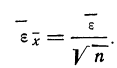
Средняя ошибка сводного результата измерения
Принимая за действительное значение измеряемой величины при равноточном измерении среднюю арифметическую из всех результатов n измерений, можно охарактеризовать точность одного измерения с помощью средней арифметической из абсолютных величин значений ошибок:
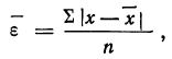
где n — число измерений, х — численное значение отдельных измерений,  — средняя арифметическая из результатов измерений.
За меру точности соответствия принятой средней арифметической  истинному значению измеряемой величины (A) принимают среднюю ошибку сводного результата измерения, вычисляемую по формуле:
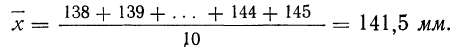
Пример 1. Произведено 10-кратное измерение размера детали (в мм), давшее следующие, расположенные в возрастающем порядке результаты: 138; 139; 140; 141; 141; 142; 142; 143; 144; 145.
Охарактеризуем сначала точность одного измерения, т. е. вычислим среднюю арифметическую из абсолютных значений ошибок. Для этой цели вычислим среднюю арифметическую из результатов измерений:
Найдем ошибки измерения:
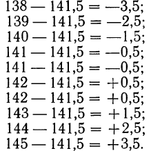
Следовательно:
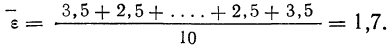
Теперь можно вычислить среднюю ошибку сводного результата измерения:
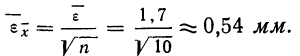
Значит, мерой точности соответствия 141,5 мм истинной величине размера детали является средняя ошибка, равная 0,54 мм.
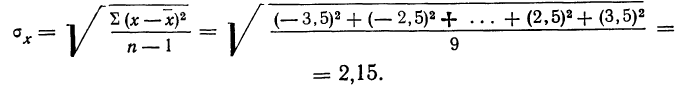
Средняя квадратическая ошибка
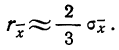
Если в качестве меры точности одного измерения принять не среднюю арифметическую из абсолютных значений ошибок (средняя ошибка), а среднюю квадратическую из ошибок измерений, т. е.
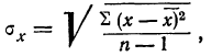
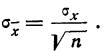
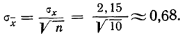
то средняя квадратическая ошибка найденной средней арифметической из ошибок измерения вычисляется по формуле:
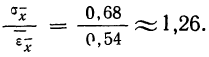
Между средней -квадратической ошибкой и средней ошибкой сводного результата измерения существует связь: 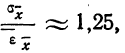 если случайные ошибки подчиняются Гауссову закону нормального распределения.
Пример 2. Используя данные предыдущего примера, находим меру точности одного измерения, т. е. среднюю квадратическую ошибку:
Затем исчисляем среднюю квадратическую ошибку найденной средней арифметической, равной 141,5 мм:
Сопоставляя среднюю квадратическую ошибку сводного результата измерения со средней ошибкой, получаем:
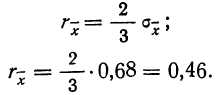
Вероятная ошибка
За меру точности одного измерения иногда принимают вероятную ошибку:
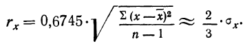
Тогда в качестве вероятной ошибки сводного результата измерения используют соотношение:
Пример 3. Используя данные предыдущих примеров, находим вероятную ошибку сводного результата измерения:
Наиболее вероятные границы сводных результатов измерения
Математическое ожидание случайной ошибки равно нулю. В качестве значения измеряемой величины применяется средняя арифметическая всех измерений (если они равноточны). Использование отклонений результатов измерений (х) от средней из них  называемых в теории ошибок «кажущимися ошибками»
  позволяет произвести оценку точности соответствия средней арифметической неизвестному истинному значению измеряемой величины (A).
Для этой цели используют удвоенную или утроенную среднюю квадратическую ошибку сводного результата измерения или его вероятную ошибку и получают:

Найденные границы неизвестной истинной величины в случае, если ошибки подчинены нормальному закону распределения Гаусса (чаще всего так и бывает), соблюдаются с большой вероятностью (0,997 и 0,954).
Пример 4. По данным предыдущих примеров находим границы истинного значения размера детали 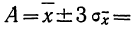
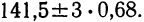 Значит, истинное значение размера детали находится в границах от 141,5—2,04 до 141,5+2,04.
- Методы математической статистики
- Комбинаторика — правила, формулы и примеры
- Классическое определение вероятности
- Геометрические вероятности
- Законы распределения случайных величин
- Дисперсионный анализ
- Математическая обработка динамических рядов
- Корреляция — определение и вычисление