Матрица ошибок keras

Create a confusion matrix for neural network predictions

In this episode, we’ll demonstrate how to create a confusion matrix, which will aid us in being able to visually observe how well a neural network is predicting during inference.

We’ll continue working with the predictions we obtained from the tf.keras.Sequential model in the
last episode.

In the
last episode, we showed how to use a trained model for inference on new data in a test set it hasn’t seen before. As mentioned in that episode, we had the labels for the test set, but we didn’t
provide these labels to the network.

Additionally, we were able to see the values that the model was predicting for each of the samples in the test set by just observing the predictions themselves.

Below are the probabilities that the model assigned to whether patients from the test set were more or less likely to experience side effects from an experimental drug.

for i in predictions:
    print(i)

[ 0.74106830  0.25893170]
[ 0.14958295  0.85041702]
[ 0.96918124  0.03081879]
[ 0.12985019  0.87014979]
[ 0.88596725  0.11403273]
...

We then looked only at the most probable prediction for each sample.

for i in rounded_predictions:
print(i)

0
1
0
1
0
...

Although we were able to read the predictions from the model easily, we weren’t easily able to compare the predictions to the true labels for the test data.

With a confusion matrix, we’ll be able to visually observe how well the model predicts on test data.

Let’s jump into the code for how this is done.

Plotting a confusion matrix

First, we import all the required libraries we’ll be working with.

%matplotlib inline
from sklearn.metrics import confusion_matrix
import itertools
import matplotlib.pyplot as plt

The confusion matrix we’ll be plotting comes from scikit-learn.

We then create the confusion matrix and assign it to the variable cm. T

cm = confusion_matrix(y_true=test_labels, y_pred=rounded_predictions)

To the confusion matrix, we pass in the true labels test_labels as well as the network’s predicted labels rounded_predictions for the test set.

Below, we have a function called plot_confusion_matrix() that came directly from
scikit-learn’s website. This is code that they provide in order to plot the confusion matrix.

def plot_confusion_matrix(cm, classes,
                        normalize=False,
                        title='Confusion matrix',
                        cmap=plt.cm.Blues):
    """
    This function prints and plots the confusion matrix.
    Normalization can be applied by setting `normalize=True`.
    """
    plt.imshow(cm, interpolation='nearest', cmap=cmap)
    plt.title(title)
    plt.colorbar()
    tick_marks = np.arange(len(classes))
    plt.xticks(tick_marks, classes, rotation=45)
    plt.yticks(tick_marks, classes)

    if normalize:
        cm = cm.astype('float') / cm.sum(axis=1)[:, np.newaxis]
        print("Normalized confusion matrix")
    else:
        print('Confusion matrix, without normalization')

    print(cm)

    thresh = cm.max() / 2.
    for i, j in itertools.product(range(cm.shape[0]), range(cm.shape[1])):
        plt.text(j, i, cm[i, j],
            horizontalalignment="center",
            color="white" if cm[i, j] > thresh else "black")

    plt.tight_layout()
    plt.ylabel('True label')
    plt.xlabel('Predicted label')

Next, we define the labels for the confusion matrix. In our case, the labels are titled “no side effects” and “had side effects.”

cm_plot_labels = ['no_side_effects','had_side_effects']

Lastly, we plot the confusion matrix by using the plot_confusion_matrix() function we just discussed. To this function, we pass in the confusion matrix cm and the labels
cm_plot_labels, as well as a title for the confusion matrix.

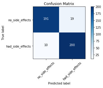
plot_confusion_matrix(cm=cm, classes=cm_plot_labels, title='Confusion Matrix')

Reading a Confusion Matrix

Looking at the plot of the confusion matrix, we have the predicted labels on the x-axis and the true labels on the y-axis. The blue cells running from the top left to bottom right contain the number of samples that the model accurately predicted. The
white cells contain the number of samples that were incorrectly predicted.

There are 420 total samples in the test set. Looking at the confusion matrix, we can see that the model accurately predicted 391 out of 420 total samples. The model
incorrectly predicted 29 out of the 420.

For the samples the model got correct, we can see that it accurately predicted that the patients would experience no side effects 191 times. It incorrectly predicted that the patient would have
no side effects 10 times when the patient did actually experience side effects.

On the other side, the model accurately predicted that the patient would experience side effects 200 times that the patient did indeed experience side effects. It incorrectly predicted that
the patient would have side effects 19 times when the patient actually did not experience side effects.

As you can see, this is a good way we can visually interpret how well the model is doing at its predictions and understand where it may need some work.