

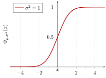
Cumulative probability of a normal distribution with expected value 0 and standard deviation 1
In statistics, the standard deviation is a measure of the amount of variation or dispersion of a set of values.[1] A low standard deviation indicates that the values tend to be close to the mean (also called the expected value) of the set, while a high standard deviation indicates that the values are spread out over a wider range.
Standard deviation may be abbreviated SD, and is most commonly represented in mathematical texts and equations by the lower case Greek letter σ (sigma), for the population standard deviation, or the Latin letter s, for the sample standard deviation.
The standard deviation of a random variable, sample, statistical population, data set, or probability distribution is the square root of its variance. It is algebraically simpler, though in practice less robust, than the average absolute deviation.[2][3] A useful property of the standard deviation is that, unlike the variance, it is expressed in the same unit as the data.
The standard deviation of a population or sample and the standard error of a statistic (e.g., of the sample mean) are quite different, but related. The sample mean’s standard error is the standard deviation of the set of means that would be found by drawing an infinite number of repeated samples from the population and computing a mean for each sample. The mean’s standard error turns out to equal the population standard deviation divided by the square root of the sample size, and is estimated by using the sample standard deviation divided by the square root of the sample size. For example, a poll’s standard error (what is reported as the margin of error of the poll), is the expected standard deviation of the estimated mean if the same poll were to be conducted multiple times. Thus, the standard error estimates the standard deviation of an estimate, which itself measures how much the estimate depends on the particular sample that was taken from the population.
In science, it is common to report both the standard deviation of the data (as a summary statistic) and the standard error of the estimate (as a measure of potential error in the findings). By convention, only effects more than two standard errors away from a null expectation are considered «statistically significant», a safeguard against spurious conclusion that is really due to random sampling error.
When only a sample of data from a population is available, the term standard deviation of the sample or sample standard deviation can refer to either the above-mentioned quantity as applied to those data, or to a modified quantity that is an unbiased estimate of the population standard deviation (the standard deviation of the entire population).
Basic examples[edit]
Population standard deviation of grades of eight students[edit]
Suppose that the entire population of interest is eight students in a particular class. For a finite set of numbers, the population standard deviation is found by taking the square root of the average of the squared deviations of the values subtracted from their average value. The marks of a class of eight students (that is, a statistical population) are the following eight values:

These eight data points have the mean (average) of 5:

First, calculate the deviations of each data point from the mean, and square the result of each:

The variance is the mean of these values:

and the population standard deviation is equal to the square root of the variance:

This formula is valid only if the eight values with which we began form the complete population. If the values instead were a random sample drawn from some large parent population (for example, they were 8 students randomly and independently chosen from a class of 2 million), then one divides by 7 (which is n − 1) instead of 8 (which is n) in the denominator of the last formula, and the result is  In that case, the result of the original formula would be called the sample standard deviation and denoted by s instead of
  Dividing by n − 1 rather than by n gives an unbiased estimate of the variance of the larger parent population. This is known as Bessel’s correction.[4][5] Roughly, the reason for it is that the formula for the sample variance relies on computing differences of observations from the sample mean, and the sample mean itself was constructed to be as close as possible to the observations, so just dividing by n would underestimate the variability.
Standard deviation of average height for adult men[edit]
If the population of interest is approximately normally distributed, the standard deviation provides information on the proportion of observations above or below certain values. For example, the average height for adult men in the United States is about 70 inches, with a standard deviation of around 3 inches. This means that most men (about 68%, assuming a normal distribution) have a height within 3 inches of the mean (67–73 inches) – one standard deviation – and almost all men (about 95%) have a height within 6 inches of the mean (64–76 inches) – two standard deviations. If the standard deviation were zero, then all men would be exactly 70 inches tall. If the standard deviation were 20 inches, then men would have much more variable heights, with a typical range of about 50–90 inches. Three standard deviations account for 99.73% of the sample population being studied, assuming the distribution is normal or bell-shaped (see the 68–95–99.7 rule, or the empirical rule, for more information).
Definition of population values[edit]
Let μ be the expected value (the average) of random variable X with density f(x):
![{displaystyle mu equiv operatorname {E} [X]=int _{-infty }^{+infty }xf(x),mathrm {d} x}](https://wikimedia.org/api/rest_v1/media/math/render/svg/fb2a61843da0d05619c0dd691dbf3fe315b395ad)
The standard deviation σ of X is defined as
![{displaystyle sigma equiv {sqrt {operatorname {E} left[(X-mu )^{2}right]}}={sqrt {int _{-infty }^{+infty }(x-mu )^{2}f(x),mathrm {d} x}},}](https://wikimedia.org/api/rest_v1/media/math/render/svg/e3a1cfef8ad100fbcae387d9581763f0b389bbc3)
which can be shown to equal ![{textstyle {sqrt {operatorname {E} left[X^{2}right]-(operatorname {E} [X])^{2}}}.}](https://wikimedia.org/api/rest_v1/media/math/render/svg/e2dd8d466c3ecb05713377fefcb7e7f787b29ce7)
Using words, the standard deviation is the square root of the variance of X.
The standard deviation of a probability distribution is the same as that of a random variable having that distribution.
Not all random variables have a standard deviation. If the distribution has fat tails going out to infinity, the standard deviation might not exist, because the integral might not converge. The normal distribution has tails going out to infinity, but its mean and standard deviation do exist, because the tails diminish quickly enough. The Pareto distribution with parameter ![{displaystyle alpha in (1,2]}](https://wikimedia.org/api/rest_v1/media/math/render/svg/782b1d598278b0238ee817c658744e8a7ed3a06e) has a mean, but not a standard deviation (loosely speaking, the standard deviation is infinite). The Cauchy distribution has neither a mean nor a standard deviation.
has a mean, but not a standard deviation (loosely speaking, the standard deviation is infinite). The Cauchy distribution has neither a mean nor a standard deviation.
Discrete random variable[edit]
In the case where X takes random values from a finite data set x1, x2, …, xN, with each value having the same probability, the standard deviation is
![{displaystyle sigma ={sqrt {{frac {1}{N}}left[(x_{1}-mu )^{2}+(x_{2}-mu )^{2}+cdots +(x_{N}-mu )^{2}right]}},{text{ where }}mu ={frac {1}{N}}(x_{1}+cdots +x_{N}),}](https://wikimedia.org/api/rest_v1/media/math/render/svg/827beb1be760eed3cb07b20d29f01d326f728071)
or, by using summation notation,

If, instead of having equal probabilities, the values have different probabilities, let x1 have probability p1, x2 have probability p2, …, xN have probability pN. In this case, the standard deviation will be

Continuous random variable[edit]
The standard deviation of a continuous real-valued random variable X with probability density function p(x) is

and where the integrals are definite integrals taken for x ranging over the set of possible values of the random variable X.
In the case of a parametric family of distributions, the standard deviation can be expressed in terms of the parameters. For example, in the case of the log-normal distribution with parameters μ and σ2, the standard deviation is

Estimation[edit]
One can find the standard deviation of an entire population in cases (such as standardized testing) where every member of a population is sampled. In cases where that cannot be done, the standard deviation σ is estimated by examining a random sample taken from the population and computing a statistic of the sample, which is used as an estimate of the population standard deviation. Such a statistic is called an estimator, and the estimator (or the value of the estimator, namely the estimate) is called a sample standard deviation, and is denoted by s (possibly with modifiers).
Unlike in the case of estimating the population mean, for which the sample mean is a simple estimator with many desirable properties (unbiased, efficient, maximum likelihood), there is no single estimator for the standard deviation with all these properties, and unbiased estimation of standard deviation is a very technically involved problem. Most often, the standard deviation is estimated using the corrected sample standard deviation (using N − 1), defined below, and this is often referred to as the «sample standard deviation», without qualifiers. However, other estimators are better in other respects: the uncorrected estimator (using N) yields lower mean squared error, while using N − 1.5 (for the normal distribution) almost completely eliminates bias.
Uncorrected sample standard deviation[edit]
The formula for the population standard deviation (of a finite population) can be applied to the sample, using the size of the sample as the size of the population (though the actual population size from which the sample is drawn may be much larger). This estimator, denoted by sN, is known as the uncorrected sample standard deviation, or sometimes the standard deviation of the sample (considered as the entire population), and is defined as follows:[6]

where  are the observed values of the sample items, and
  is the mean value of these observations, while the denominator N stands for the size of the sample: this is the square root of the sample variance, which is the average of the squared deviations about the sample mean.
This is a consistent estimator (it converges in probability to the population value as the number of samples goes to infinity), and is the maximum-likelihood estimate when the population is normally distributed.[7] However, this is a biased estimator, as the estimates are generally too low. The bias decreases as sample size grows, dropping off as 1/N, and thus is most significant for small or moderate sample sizes; for  the bias is below 1%. Thus for very large sample sizes, the uncorrected sample standard deviation is generally acceptable. This estimator also has a uniformly smaller mean squared error than the corrected sample standard deviation.
Corrected sample standard deviation[edit]
If the biased sample variance (the second central moment of the sample, which is a downward-biased estimate of the population variance) is used to compute an estimate of the population’s standard deviation, the result is

Here taking the square root introduces further downward bias, by Jensen’s inequality, due to the square root’s being a concave function. The bias in the variance is easily corrected, but the bias from the square root is more difficult to correct, and depends on the distribution in question.
An unbiased estimator for the variance is given by applying Bessel’s correction, using N − 1 instead of N to yield the unbiased sample variance, denoted s2:

This estimator is unbiased if the variance exists and the sample values are drawn independently with replacement. N − 1 corresponds to the number of degrees of freedom in the vector of deviations from the mean, 
Taking square roots reintroduces bias (because the square root is a nonlinear function which does not commute with the expectation, i.e. often ![{displaystyle E[{sqrt {X}}]neq {sqrt {E[X]}}}](https://wikimedia.org/api/rest_v1/media/math/render/svg/79fa5d2ba8891a41598ddeadc10ba844a20cdfa0) ), yielding the corrected sample standard deviation, denoted by s:
), yielding the corrected sample standard deviation, denoted by s:

As explained above, while s2 is an unbiased estimator for the population variance, s is still a biased estimator for the population standard deviation, though markedly less biased than the uncorrected sample standard deviation. This estimator is commonly used and generally known simply as the «sample standard deviation». The bias may still be large for small samples (N less than 10). As sample size increases, the amount of bias decreases. We obtain more information and the difference between  and
and  becomes smaller.
Unbiased sample standard deviation[edit]
For unbiased estimation of standard deviation, there is no formula that works across all distributions, unlike for mean and variance. Instead, s is used as a basis, and is scaled by a correction factor to produce an unbiased estimate. For the normal distribution, an unbiased estimator is given by s/c4, where the correction factor (which depends on N) is given in terms of the Gamma function, and equals:

This arises because the sampling distribution of the sample standard deviation follows a (scaled) chi distribution, and the correction factor is the mean of the chi distribution.
An approximation can be given by replacing N − 1 with N − 1.5, yielding:

The error in this approximation decays quadratically (as 1/N2), and it is suited for all but the smallest samples or highest precision: for N = 3 the bias is equal to 1.3%, and for N = 9 the bias is already less than 0.1%.
A more accurate approximation is to replace  above with
  .[8]
.[8]
For other distributions, the correct formula depends on the distribution, but a rule of thumb is to use the further refinement of the approximation:

where γ2 denotes the population excess kurtosis. The excess kurtosis may be either known beforehand for certain distributions, or estimated from the data.[9]
Confidence interval of a sampled standard deviation[edit]
The standard deviation we obtain by sampling a distribution is itself not absolutely accurate, both for mathematical reasons (explained here by the confidence interval) and for practical reasons of measurement (measurement error). The mathematical effect can be described by the confidence interval or CI.
To show how a larger sample will make the confidence interval narrower, consider the following examples:
A small population of N = 2 has only 1 degree of freedom for estimating the standard deviation. The result is that a 95% CI of the SD runs from 0.45 × SD to 31.9 × SD; the factors here are as follows:

where  is the p-th quantile of the chi-square distribution with k degrees of freedom, and
  is the confidence level. This is equivalent to the following:

With k = 1,  and
and  . The reciprocals of the square roots of these two numbers give us the factors 0.45 and 31.9 given above.
A larger population of N = 10 has 9 degrees of freedom for estimating the standard deviation. The same computations as above give us in this case a 95% CI running from 0.69 × SD to 1.83 × SD. So even with a sample population of 10, the actual SD can still be almost a factor 2 higher than the sampled SD. For a sample population N=100, this is down to 0.88 × SD to 1.16 × SD. To be more certain that the sampled SD is close to the actual SD we need to sample a large number of points.
These same formulae can be used to obtain confidence intervals on the variance of residuals from a least squares fit under standard normal theory, where k is now the number of degrees of freedom for error.
Bounds on standard deviation[edit]
For a set of N > 4 data spanning a range of values R, an upper bound on the standard deviation s is given by s = 0.6R.[10]
An estimate of the standard deviation for N > 100 data taken to be approximately normal follows from the heuristic that 95% of the area under the normal curve lies roughly two standard deviations to either side of the mean, so that, with 95% probability the total range of values R represents four standard deviations so that s ≈ R/4. This so-called range rule is useful in sample size estimation, as the range of possible values is easier to estimate than the standard deviation. Other divisors K(N) of the range such that s ≈ R/K(N) are available for other values of N and for non-normal distributions.[11]
Identities and mathematical properties[edit]
The standard deviation is invariant under changes in location, and scales directly with the scale of the random variable. Thus, for a constant c and random variables X and Y:

The standard deviation of the sum of two random variables can be related to their individual standard deviations and the covariance between them:

where  and
and  stand for variance and covariance, respectively.
The calculation of the sum of squared deviations can be related to moments calculated directly from the data. In the following formula, the letter E is interpreted to mean expected value, i.e., mean.
![{displaystyle sigma (X)={sqrt {operatorname {E} left[(X-operatorname {E} [X])^{2}right]}}={sqrt {operatorname {E} left[X^{2}right]-(operatorname {E} [X])^{2}}}.}](https://wikimedia.org/api/rest_v1/media/math/render/svg/d3ab12089bd2027790ef060ff7cc2ec05ae2021f)
The sample standard deviation can be computed as:
![{displaystyle s(X)={sqrt {frac {N}{N-1}}}{sqrt {operatorname {E} left[(X-operatorname {E} [X])^{2}right]}}.}](https://wikimedia.org/api/rest_v1/media/math/render/svg/702e9da21c721697e6e81932bf8b7443028f7d6d)
For a finite population with equal probabilities at all points, we have

which means that the standard deviation is equal to the square root of the difference between the average of the squares of the values and the square of the average value.
See computational formula for the variance for proof, and for an analogous result for the sample standard deviation.
Interpretation and application[edit]

Example of samples from two populations with the same mean but different standard deviations. Red population has mean 100 and SD 10; blue population has mean 100 and SD 50.
A large standard deviation indicates that the data points can spread far from the mean and a small standard deviation indicates that they are clustered closely around the mean.
For example, each of the three populations {0, 0, 14, 14}, {0, 6, 8, 14} and {6, 6, 8, 8} has a mean of 7. Their standard deviations are 7, 5, and 1, respectively. The third population has a much smaller standard deviation than the other two because its values are all close to 7. These standard deviations have the same units as the data points themselves. If, for instance, the data set {0, 6, 8, 14} represents the ages of a population of four siblings in years, the standard deviation is 5 years. As another example, the population {1000, 1006, 1008, 1014} may represent the distances traveled by four athletes, measured in meters. It has a mean of 1007 meters, and a standard deviation of 5 meters.
Standard deviation may serve as a measure of uncertainty. In physical science, for example, the reported standard deviation of a group of repeated measurements gives the precision of those measurements. When deciding whether measurements agree with a theoretical prediction, the standard deviation of those measurements is of crucial importance: if the mean of the measurements is too far away from the prediction (with the distance measured in standard deviations), then the theory being tested probably needs to be revised. This makes sense since they fall outside the range of values that could reasonably be expected to occur, if the prediction were correct and the standard deviation appropriately quantified. See prediction interval.
While the standard deviation does measure how far typical values tend to be from the mean, other measures are available. An example is the mean absolute deviation, which might be considered a more direct measure of average distance, compared to the root mean square distance inherent in the standard deviation.
Application examples[edit]
The practical value of understanding the standard deviation of a set of values is in appreciating how much variation there is from the average (mean).
Experiment, industrial and hypothesis testing[edit]
Standard deviation is often used to compare real-world data against a model to test the model.
For example, in industrial applications the weight of products coming off a production line may need to comply with a legally required value. By weighing some fraction of the products an average weight can be found, which will always be slightly different from the long-term average. By using standard deviations, a minimum and maximum value can be calculated that the averaged weight will be within some very high percentage of the time (99.9% or more). If it falls outside the range then the production process may need to be corrected. Statistical tests such as these are particularly important when the testing is relatively expensive. For example, if the product needs to be opened and drained and weighed, or if the product was otherwise used up by the test.
In experimental science, a theoretical model of reality is used. Particle physics conventionally uses a standard of «5 sigma» for the declaration of a discovery. A five-sigma level translates to one chance in 3.5 million that a random fluctuation would yield the result. This level of certainty was required in order to assert that a particle consistent with the Higgs boson had been discovered in two independent experiments at CERN,[12] also leading to the declaration of the first observation of gravitational waves.[13]
Weather[edit]
As a simple example, consider the average daily maximum temperatures for two cities, one inland and one on the coast. It is helpful to understand that the range of daily maximum temperatures for cities near the coast is smaller than for cities inland. Thus, while these two cities may each have the same average maximum temperature, the standard deviation of the daily maximum temperature for the coastal city will be less than that of the inland city as, on any particular day, the actual maximum temperature is more likely to be farther from the average maximum temperature for the inland city than for the coastal one.
Finance[edit]
In finance, standard deviation is often used as a measure of the risk associated with price-fluctuations of a given asset (stocks, bonds, property, etc.), or the risk of a portfolio of assets[14] (actively managed mutual funds, index mutual funds, or ETFs). Risk is an important factor in determining how to efficiently manage a portfolio of investments because it determines the variation in returns on the asset and/or portfolio and gives investors a mathematical basis for investment decisions (known as mean-variance optimization). The fundamental concept of risk is that as it increases, the expected return on an investment should increase as well, an increase known as the risk premium. In other words, investors should expect a higher return on an investment when that investment carries a higher level of risk or uncertainty. When evaluating investments, investors should estimate both the expected return and the uncertainty of future returns. Standard deviation provides a quantified estimate of the uncertainty of future returns.
For example, assume an investor had to choose between two stocks. Stock A over the past 20 years had an average return of 10 percent, with a standard deviation of 20 percentage points (pp) and Stock B, over the same period, had average returns of 12 percent but a higher standard deviation of 30 pp. On the basis of risk and return, an investor may decide that Stock A is the safer choice, because Stock B’s additional two percentage points of return is not worth the additional 10 pp standard deviation (greater risk or uncertainty of the expected return). Stock B is likely to fall short of the initial investment (but also to exceed the initial investment) more often than Stock A under the same circumstances, and is estimated to return only two percent more on average. In this example, Stock A is expected to earn about 10 percent, plus or minus 20 pp (a range of 30 percent to −10 percent), about two-thirds of the future year returns. When considering more extreme possible returns or outcomes in future, an investor should expect results of as much as 10 percent plus or minus 60 pp, or a range from 70 percent to −50 percent, which includes outcomes for three standard deviations from the average return (about 99.7 percent of probable returns).
Calculating the average (or arithmetic mean) of the return of a security over a given period will generate the expected return of the asset. For each period, subtracting the expected return from the actual return results in the difference from the mean. Squaring the difference in each period and taking the average gives the overall variance of the return of the asset. The larger the variance, the greater risk the security carries. Finding the square root of this variance will give the standard deviation of the investment tool in question.
Population standard deviation is used to set the width of Bollinger Bands, a technical analysis tool. For example, the upper Bollinger Band is given as  The most commonly used value for n is 2; there is about a five percent chance of going outside, assuming a normal distribution of returns.
Financial time series are known to be non-stationary series, whereas the statistical calculations above, such as standard deviation, apply only to stationary series. To apply the above statistical tools to non-stationary series, the series first must be transformed to a stationary series, enabling use of statistical tools that now have a valid basis from which to work.
Geometric interpretation[edit]
To gain some geometric insights and clarification, we will start with a population of three values, x1, x2, x3. This defines a point P = (x1, x2, x3) in R3. Consider the line L = {(r, r, r) : r ∈ R}. This is the «main diagonal» going through the origin. If our three given values were all equal, then the standard deviation would be zero and P would lie on L. So it is not unreasonable to assume that the standard deviation is related to the distance of P to L. That is indeed the case. To move orthogonally from L to the point P, one begins at the point:

whose coordinates are the mean of the values we started out with.
A little algebra shows that the distance between P and M (which is the same as the orthogonal distance between P and the line L)  is equal to the standard deviation of the vector (x1, x2, x3), multiplied by the square root of the number of dimensions of the vector (3 in this case).
Chebyshev’s inequality[edit]
An observation is rarely more than a few standard deviations away from the mean. Chebyshev’s inequality ensures that, for all distributions for which the standard deviation is defined, the amount of data within a number of standard deviations of the mean is at least as much as given in the following table.
| Distance from mean | Minimum population |
|---|---|
 |
50% |
| 2σ | 75% |
| 3σ | 89% |
| 4σ | 94% |
| 5σ | 96% |
| 6σ | 97% |
 |
 [15] [15]
|
 |

|
Rules for normally distributed data[edit]
Dark blue is one standard deviation on either side of the mean. For the normal distribution, this accounts for 68.27 percent of the set; while two standard deviations from the mean (medium and dark blue) account for 95.45 percent; three standard deviations (light, medium, and dark blue) account for 99.73 percent; and four standard deviations account for 99.994 percent. The two points of the curve that are one standard deviation from the mean are also the inflection points.
The central limit theorem states that the distribution of an average of many independent, identically distributed random variables tends toward the famous bell-shaped normal distribution with a probability density function of

where μ is the expected value of the random variables, σ equals their distribution’s standard deviation divided by n1/2, and n is the number of random variables. The standard deviation therefore is simply a scaling variable that adjusts how broad the curve will be, though it also appears in the normalizing constant.
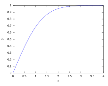
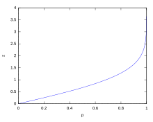
If a data distribution is approximately normal, then the proportion of data values within z standard deviations of the mean is defined by:

where  is the error function. The proportion that is less than or equal to a number, x, is given by the cumulative distribution function:
![{displaystyle {text{Proportion}}leq x={frac {1}{2}}left[1+operatorname {erf} left({frac {x-mu }{sigma {sqrt {2}}}}right)right]={frac {1}{2}}left[1+operatorname {erf} left({frac {z}{sqrt {2}}}right)right]}](data:image/svg+xml,%3Csvg%20xmlns='http://www.w3.org/2000/svg'%20viewBox='0%200%200%200'%3E%3C/svg%3E) .[16]
.[16]
![{displaystyle {text{Proportion}}leq x={frac {1}{2}}left[1+operatorname {erf} left({frac {x-mu }{sigma {sqrt {2}}}}right)right]={frac {1}{2}}left[1+operatorname {erf} left({frac {z}{sqrt {2}}}right)right]}](https://wikimedia.org/api/rest_v1/media/math/render/svg/3907d1b0502235fa3fd00f261b290406a02e7b21)
If a data distribution is approximately normal then about 68 percent of the data values are within one standard deviation of the mean (mathematically, μ ± σ, where μ is the arithmetic mean), about 95 percent are within two standard deviations (μ ± 2σ), and about 99.7 percent lie within three standard deviations (μ ± 3σ). This is known as the 68–95–99.7 rule, or the empirical rule.
For various values of z, the percentage of values expected to lie in and outside the symmetric interval, CI = (−zσ, zσ), are as follows:
| Confidence interval |
Proportion within | Proportion without | |
|---|---|---|---|
| Percentage | Percentage | Fraction | |
| 0.318639σ | 25% | 75% | 3 / 4 |
| 0.674490σ | 50% | 50% | 1 / 2 |
| 0.977925σ | 66.6667% | 33.3333% | 1 / 3 |
| 0.994458σ | 68% | 32% | 1 / 3.125 |
| 1σ | 68.2689492% | 31.7310508% | 1 / 3.1514872 |
| 1.281552σ | 80% | 20% | 1 / 5 |
| 1.644854σ | 90% | 10% | 1 / 10 |
| 1.959964σ | 95% | 5% | 1 / 20 |
| 2σ | 95.4499736% | 4.5500264% | 1 / 21.977895 |
| 2.575829σ | 99% | 1% | 1 / 100 |
| 3σ | 99.7300204% | 0.2699796% | 1 / 370.398 |
| 3.290527σ | 99.9% | 0.1% | 1 / 1000 |
| 3.890592σ | 99.99% | 0.01% | 1 / 10000 |
| 4σ | 99.993666% | 0.006334% | 1 / 15787 |
| 4.417173σ | 99.999% | 0.001% | 1 / 100000 |
| 4.5σ | 99.9993204653751% | 0.0006795346249% | 1 / 147159.5358 6.8 / 1000000 |
| 4.891638σ | 99.9999% | 0.0001% | 1 / 1000000 |
| 5σ | 99.9999426697% | 0.0000573303% | 1 / 1744278 |
| 5.326724σ | 99.99999% | 0.00001% | 1 / 10000000 |
| 5.730729σ | 99.999999% | 0.000001% | 1 / 100000000 |
| 6σ | 99.9999998027% | 0.0000001973% | 1 / 506797346 |
| 6.109410σ | 99.9999999% | 0.0000001% | 1 / 1000000000 |
| 6.466951σ | 99.99999999% | 0.00000001% | 1 / 10000000000 |
| 6.806502σ | 99.999999999% | 0.000000001% | 1 / 100000000000 |
| 7σ | 99.9999999997440% | 0.000000000256% | 1 / 390682215445 |
Relationship between standard deviation and mean[edit]
The mean and the standard deviation of a set of data are descriptive statistics usually reported together. In a certain sense, the standard deviation is a «natural» measure of statistical dispersion if the center of the data is measured about the mean. This is because the standard deviation from the mean is smaller than from any other point. The precise statement is the following: suppose x1, …, xn are real numbers and define the function:

Using calculus or by completing the square, it is possible to show that σ(r) has a unique minimum at the mean:

Variability can also be measured by the coefficient of variation, which is the ratio of the standard deviation to the mean. It is a dimensionless number.
Standard deviation of the mean[edit]
Often, we want some information about the precision of the mean we obtained. We can obtain this by determining the standard deviation of the sampled mean. Assuming statistical independence of the values in the sample, the standard deviation of the mean is related to the standard deviation of the distribution by:

where N is the number of observations in the sample used to estimate the mean. This can easily be proven with (see basic properties of the variance):

(Statistical independence is assumed.)

hence

Resulting in:

In order to estimate the standard deviation of the mean  it is necessary to know the standard deviation of the entire population
  beforehand. However, in most applications this parameter is unknown. For example, if a series of 10 measurements of a previously unknown quantity is performed in a laboratory, it is possible to calculate the resulting sample mean and sample standard deviation, but it is impossible to calculate the standard deviation of the mean. However, one can estimate the standard deviation of the entire population from the sample, and thus obtain an estimate for the standard error of the mean.
Rapid calculation methods[edit]
The following two formulas can represent a running (repeatedly updated) standard deviation. A set of two power sums s1 and s2 are computed over a set of N values of x, denoted as x1, …, xN:

Given the results of these running summations, the values N, s1, s2 can be used at any time to compute the current value of the running standard deviation:

Where N, as mentioned above, is the size of the set of values (or can also be regarded as s0).
Similarly for sample standard deviation,

In a computer implementation, as the two sj sums become large, we need to consider round-off error, arithmetic overflow, and arithmetic underflow. The method below calculates the running sums method with reduced rounding errors.[17] This is a «one pass» algorithm for calculating variance of n samples without the need to store prior data during the calculation. Applying this method to a time series will result in successive values of standard deviation corresponding to n data points as n grows larger with each new sample, rather than a constant-width sliding window calculation.
For k = 1, …, n:

where A is the mean value.

Note:  since
since  or
or 
Sample variance:

Population variance:

Weighted calculation[edit]
When the values xi are weighted with unequal weights wi, the power sums s0, s1, s2 are each computed as:

And the standard deviation equations remain unchanged. s0 is now the sum of the weights and not the number of samples N.
The incremental method with reduced rounding errors can also be applied, with some additional complexity.
A running sum of weights must be computed for each k from 1 to n:

and places where 1/n is used above must be replaced by wi/Wn:

In the final division,

and

or

where n is the total number of elements, and n’ is the number of elements with non-zero weights.
The above formulas become equal to the simpler formulas given above if weights are taken as equal to one.
History[edit]
The term standard deviation was first used in writing by Karl Pearson in 1894, following his use of it in lectures.[18][19] This was as a replacement for earlier alternative names for the same idea: for example, Gauss used mean error.[20]
Higher dimensions[edit]
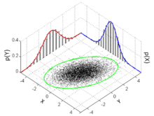
The standard deviation ellipse (green) of a two-dimensional normal distribution
In two dimensions, the standard deviation can be illustrated with the standard deviation ellipse (see Multivariate normal distribution § Geometric interpretation).
See also[edit]
- 68–95–99.7 rule
- Accuracy and precision
- Chebyshev’s inequality An inequality on location and scale parameters
- Coefficient of variation
- Cumulant
- Deviation (statistics)
- Distance correlation Distance standard deviation
- Error bar
- Geometric standard deviation
- Mahalanobis distance generalizing number of standard deviations to the mean
- Mean absolute error
- Pooled variance
- Propagation of uncertainty
- Percentile
- Raw data
- Robust standard deviation
- Root mean square
- Sample size
- Samuelson’s inequality
- Six Sigma
- Standard error
- Standard score
- Yamartino method for calculating standard deviation of wind direction
References[edit]
- ^ Bland, J.M.; Altman, D.G. (1996). «Statistics notes: measurement error». BMJ. 312 (7047): 1654. doi:10.1136/bmj.312.7047.1654. PMC 2351401. PMID 8664723.
- ^ Gauss, Carl Friedrich (1816). «Bestimmung der Genauigkeit der Beobachtungen». Zeitschrift für Astronomie und Verwandte Wissenschaften. 1: 187–197.
- ^ Walker, Helen (1931). Studies in the History of the Statistical Method. Baltimore, MD: Williams & Wilkins Co. pp. 24–25.
- ^ Weisstein, Eric W. «Bessel’s Correction». MathWorld.
- ^ «Standard Deviation Formulas». www.mathsisfun.com. Retrieved 21 August 2020.
- ^ Weisstein, Eric W. «Standard Deviation». mathworld.wolfram.com. Retrieved 21 August 2020.
- ^ «Consistent estimator». www.statlect.com. Retrieved 10 October 2022.
- ^ Gurland, John; Tripathi, Ram C. (1971), «A Simple Approximation for Unbiased Estimation of the Standard Deviation», The American Statistician, 25 (4): 30–32, doi:10.2307/2682923, JSTOR 2682923
- ^ «Standard Deviation Calculator». PureCalculators. 11 July 2021. Retrieved 14 September 2021.
- ^ Shiffler, Ronald E.; Harsha, Phillip D. (1980). «Upper and Lower Bounds for the Sample Standard Deviation». Teaching Statistics. 2 (3): 84–86. doi:10.1111/j.1467-9639.1980.tb00398.x.
- ^ Browne, Richard H. (2001). «Using the Sample Range as a Basis for Calculating Sample Size in Power Calculations». The American Statistician. 55 (4): 293–298. doi:10.1198/000313001753272420. JSTOR 2685690. S2CID 122328846.
- ^ «CERN experiments observe particle consistent with long-sought Higgs boson | CERN press office». Press.web.cern.ch. 4 July 2012. Archived from the original on 25 March 2016. Retrieved 30 May 2015.
- ^ LIGO Scientific Collaboration, Virgo Collaboration (2016), «Observation of Gravitational Waves from a Binary Black Hole Merger», Physical Review Letters, 116 (6): 061102, arXiv:1602.03837, Bibcode:2016PhRvL.116f1102A, doi:10.1103/PhysRevLett.116.061102, PMID 26918975, S2CID 124959784
- ^ «What is Standard Deviation». Pristine. Retrieved 29 October 2011.
- ^ Ghahramani, Saeed (2000). Fundamentals of Probability (2nd ed.). New Jersey: Prentice Hall. p. 438. ISBN 9780130113290.
- ^ Eric W. Weisstein. «Distribution Function». MathWorld—A Wolfram Web Resource. Retrieved 30 September 2014.
- ^ Welford, BP (August 1962). «Note on a Method for Calculating Corrected Sums of Squares and Products». Technometrics. 4 (3): 419–420. CiteSeerX 10.1.1.302.7503. doi:10.1080/00401706.1962.10490022.
- ^ Dodge, Yadolah (2003). The Oxford Dictionary of Statistical Terms. Oxford University Press. ISBN 978-0-19-920613-1.
- ^ Pearson, Karl (1894). «On the dissection of asymmetrical frequency curves». Philosophical Transactions of the Royal Society A. 185: 71–110. Bibcode:1894RSPTA.185…71P. doi:10.1098/rsta.1894.0003.
- ^ Miller, Jeff. «Earliest Known Uses of Some of the Words of Mathematics».
External links[edit]
- «Quadratic deviation», Encyclopedia of Mathematics, EMS Press, 2001 [1994]
- «Standard Deviation Calculator»
Cumulative probability of a normal distribution with expected value 0 and standard deviation 1
In statistics, the standard deviation is a measure of the amount of variation or dispersion of a set of values.[1] A low standard deviation indicates that the values tend to be close to the mean (also called the expected value) of the set, while a high standard deviation indicates that the values are spread out over a wider range.
Standard deviation may be abbreviated SD, and is most commonly represented in mathematical texts and equations by the lower case Greek letter σ (sigma), for the population standard deviation, or the Latin letter s, for the sample standard deviation.
The standard deviation of a random variable, sample, statistical population, data set, or probability distribution is the square root of its variance. It is algebraically simpler, though in practice less robust, than the average absolute deviation.[2][3] A useful property of the standard deviation is that, unlike the variance, it is expressed in the same unit as the data.
The standard deviation of a population or sample and the standard error of a statistic (e.g., of the sample mean) are quite different, but related. The sample mean’s standard error is the standard deviation of the set of means that would be found by drawing an infinite number of repeated samples from the population and computing a mean for each sample. The mean’s standard error turns out to equal the population standard deviation divided by the square root of the sample size, and is estimated by using the sample standard deviation divided by the square root of the sample size. For example, a poll’s standard error (what is reported as the margin of error of the poll), is the expected standard deviation of the estimated mean if the same poll were to be conducted multiple times. Thus, the standard error estimates the standard deviation of an estimate, which itself measures how much the estimate depends on the particular sample that was taken from the population.
In science, it is common to report both the standard deviation of the data (as a summary statistic) and the standard error of the estimate (as a measure of potential error in the findings). By convention, only effects more than two standard errors away from a null expectation are considered «statistically significant», a safeguard against spurious conclusion that is really due to random sampling error.
When only a sample of data from a population is available, the term standard deviation of the sample or sample standard deviation can refer to either the above-mentioned quantity as applied to those data, or to a modified quantity that is an unbiased estimate of the population standard deviation (the standard deviation of the entire population).
Basic examples[edit]
Population standard deviation of grades of eight students[edit]
Suppose that the entire population of interest is eight students in a particular class. For a finite set of numbers, the population standard deviation is found by taking the square root of the average of the squared deviations of the values subtracted from their average value. The marks of a class of eight students (that is, a statistical population) are the following eight values:
These eight data points have the mean (average) of 5:
First, calculate the deviations of each data point from the mean, and square the result of each:
The variance is the mean of these values:
and the population standard deviation is equal to the square root of the variance:
This formula is valid only if the eight values with which we began form the complete population. If the values instead were a random sample drawn from some large parent population (for example, they were 8 students randomly and independently chosen from a class of 2 million), then one divides by 7 (which is n − 1) instead of 8 (which is n) in the denominator of the last formula, and the result is In that case, the result of the original formula would be called the sample standard deviation and denoted by s instead of Dividing by n − 1 rather than by n gives an unbiased estimate of the variance of the larger parent population. This is known as Bessel’s correction.[4][5] Roughly, the reason for it is that the formula for the sample variance relies on computing differences of observations from the sample mean, and the sample mean itself was constructed to be as close as possible to the observations, so just dividing by n would underestimate the variability.
Standard deviation of average height for adult men[edit]
If the population of interest is approximately normally distributed, the standard deviation provides information on the proportion of observations above or below certain values. For example, the average height for adult men in the United States is about 70 inches, with a standard deviation of around 3 inches. This means that most men (about 68%, assuming a normal distribution) have a height within 3 inches of the mean (67–73 inches) – one standard deviation – and almost all men (about 95%) have a height within 6 inches of the mean (64–76 inches) – two standard deviations. If the standard deviation were zero, then all men would be exactly 70 inches tall. If the standard deviation were 20 inches, then men would have much more variable heights, with a typical range of about 50–90 inches. Three standard deviations account for 99.73% of the sample population being studied, assuming the distribution is normal or bell-shaped (see the 68–95–99.7 rule, or the empirical rule, for more information).
Definition of population values[edit]
Let μ be the expected value (the average) of random variable X with density f(x):
The standard deviation σ of X is defined as
which can be shown to equal
Using words, the standard deviation is the square root of the variance of X.
The standard deviation of a probability distribution is the same as that of a random variable having that distribution.
Not all random variables have a standard deviation. If the distribution has fat tails going out to infinity, the standard deviation might not exist, because the integral might not converge. The normal distribution has tails going out to infinity, but its mean and standard deviation do exist, because the tails diminish quickly enough. The Pareto distribution with parameter has a mean, but not a standard deviation (loosely speaking, the standard deviation is infinite). The Cauchy distribution has neither a mean nor a standard deviation.
Discrete random variable[edit]
In the case where X takes random values from a finite data set x1, x2, …, xN, with each value having the same probability, the standard deviation is
or, by using summation notation,
If, instead of having equal probabilities, the values have different probabilities, let x1 have probability p1, x2 have probability p2, …, xN have probability pN. In this case, the standard deviation will be
Continuous random variable[edit]
The standard deviation of a continuous real-valued random variable X with probability density function p(x) is
and where the integrals are definite integrals taken for x ranging over the set of possible values of the random variable X.
In the case of a parametric family of distributions, the standard deviation can be expressed in terms of the parameters. For example, in the case of the log-normal distribution with parameters μ and σ2, the standard deviation is
Estimation[edit]
One can find the standard deviation of an entire population in cases (such as standardized testing) where every member of a population is sampled. In cases where that cannot be done, the standard deviation σ is estimated by examining a random sample taken from the population and computing a statistic of the sample, which is used as an estimate of the population standard deviation. Such a statistic is called an estimator, and the estimator (or the value of the estimator, namely the estimate) is called a sample standard deviation, and is denoted by s (possibly with modifiers).
Unlike in the case of estimating the population mean, for which the sample mean is a simple estimator with many desirable properties (unbiased, efficient, maximum likelihood), there is no single estimator for the standard deviation with all these properties, and unbiased estimation of standard deviation is a very technically involved problem. Most often, the standard deviation is estimated using the corrected sample standard deviation (using N − 1), defined below, and this is often referred to as the «sample standard deviation», without qualifiers. However, other estimators are better in other respects: the uncorrected estimator (using N) yields lower mean squared error, while using N − 1.5 (for the normal distribution) almost completely eliminates bias.
Uncorrected sample standard deviation[edit]
The formula for the population standard deviation (of a finite population) can be applied to the sample, using the size of the sample as the size of the population (though the actual population size from which the sample is drawn may be much larger). This estimator, denoted by sN, is known as the uncorrected sample standard deviation, or sometimes the standard deviation of the sample (considered as the entire population), and is defined as follows:[6]
where are the observed values of the sample items, and is the mean value of these observations, while the denominator N stands for the size of the sample: this is the square root of the sample variance, which is the average of the squared deviations about the sample mean.
This is a consistent estimator (it converges in probability to the population value as the number of samples goes to infinity), and is the maximum-likelihood estimate when the population is normally distributed.[7] However, this is a biased estimator, as the estimates are generally too low. The bias decreases as sample size grows, dropping off as 1/N, and thus is most significant for small or moderate sample sizes; for the bias is below 1%. Thus for very large sample sizes, the uncorrected sample standard deviation is generally acceptable. This estimator also has a uniformly smaller mean squared error than the corrected sample standard deviation.
Corrected sample standard deviation[edit]
If the biased sample variance (the second central moment of the sample, which is a downward-biased estimate of the population variance) is used to compute an estimate of the population’s standard deviation, the result is
Here taking the square root introduces further downward bias, by Jensen’s inequality, due to the square root’s being a concave function. The bias in the variance is easily corrected, but the bias from the square root is more difficult to correct, and depends on the distribution in question.
An unbiased estimator for the variance is given by applying Bessel’s correction, using N − 1 instead of N to yield the unbiased sample variance, denoted s2:
This estimator is unbiased if the variance exists and the sample values are drawn independently with replacement. N − 1 corresponds to the number of degrees of freedom in the vector of deviations from the mean,
Taking square roots reintroduces bias (because the square root is a nonlinear function which does not commute with the expectation, i.e. often ), yielding the corrected sample standard deviation, denoted by s:
As explained above, while s2 is an unbiased estimator for the population variance, s is still a biased estimator for the population standard deviation, though markedly less biased than the uncorrected sample standard deviation. This estimator is commonly used and generally known simply as the «sample standard deviation». The bias may still be large for small samples (N less than 10). As sample size increases, the amount of bias decreases. We obtain more information and the difference between and becomes smaller.
Unbiased sample standard deviation[edit]
For unbiased estimation of standard deviation, there is no formula that works across all distributions, unlike for mean and variance. Instead, s is used as a basis, and is scaled by a correction factor to produce an unbiased estimate. For the normal distribution, an unbiased estimator is given by s/c4, where the correction factor (which depends on N) is given in terms of the Gamma function, and equals:
This arises because the sampling distribution of the sample standard deviation follows a (scaled) chi distribution, and the correction factor is the mean of the chi distribution.
An approximation can be given by replacing N − 1 with N − 1.5, yielding:
The error in this approximation decays quadratically (as 1/N2), and it is suited for all but the smallest samples or highest precision: for N = 3 the bias is equal to 1.3%, and for N = 9 the bias is already less than 0.1%.
A more accurate approximation is to replace above with .[8]
For other distributions, the correct formula depends on the distribution, but a rule of thumb is to use the further refinement of the approximation:
where γ2 denotes the population excess kurtosis. The excess kurtosis may be either known beforehand for certain distributions, or estimated from the data.[9]
Confidence interval of a sampled standard deviation[edit]
The standard deviation we obtain by sampling a distribution is itself not absolutely accurate, both for mathematical reasons (explained here by the confidence interval) and for practical reasons of measurement (measurement error). The mathematical effect can be described by the confidence interval or CI.
To show how a larger sample will make the confidence interval narrower, consider the following examples:
A small population of N = 2 has only 1 degree of freedom for estimating the standard deviation. The result is that a 95% CI of the SD runs from 0.45 × SD to 31.9 × SD; the factors here are as follows:
where is the p-th quantile of the chi-square distribution with k degrees of freedom, and is the confidence level. This is equivalent to the following:
With k = 1, and . The reciprocals of the square roots of these two numbers give us the factors 0.45 and 31.9 given above.
A larger population of N = 10 has 9 degrees of freedom for estimating the standard deviation. The same computations as above give us in this case a 95% CI running from 0.69 × SD to 1.83 × SD. So even with a sample population of 10, the actual SD can still be almost a factor 2 higher than the sampled SD. For a sample population N=100, this is down to 0.88 × SD to 1.16 × SD. To be more certain that the sampled SD is close to the actual SD we need to sample a large number of points.
These same formulae can be used to obtain confidence intervals on the variance of residuals from a least squares fit under standard normal theory, where k is now the number of degrees of freedom for error.
Bounds on standard deviation[edit]
For a set of N > 4 data spanning a range of values R, an upper bound on the standard deviation s is given by s = 0.6R.[10]
An estimate of the standard deviation for N > 100 data taken to be approximately normal follows from the heuristic that 95% of the area under the normal curve lies roughly two standard deviations to either side of the mean, so that, with 95% probability the total range of values R represents four standard deviations so that s ≈ R/4. This so-called range rule is useful in sample size estimation, as the range of possible values is easier to estimate than the standard deviation. Other divisors K(N) of the range such that s ≈ R/K(N) are available for other values of N and for non-normal distributions.[11]
Identities and mathematical properties[edit]
The standard deviation is invariant under changes in location, and scales directly with the scale of the random variable. Thus, for a constant c and random variables X and Y:
The standard deviation of the sum of two random variables can be related to their individual standard deviations and the covariance between them:
where and stand for variance and covariance, respectively.
The calculation of the sum of squared deviations can be related to moments calculated directly from the data. In the following formula, the letter E is interpreted to mean expected value, i.e., mean.
The sample standard deviation can be computed as:
For a finite population with equal probabilities at all points, we have
which means that the standard deviation is equal to the square root of the difference between the average of the squares of the values and the square of the average value.
See computational formula for the variance for proof, and for an analogous result for the sample standard deviation.
Interpretation and application[edit]
Example of samples from two populations with the same mean but different standard deviations. Red population has mean 100 and SD 10; blue population has mean 100 and SD 50.
A large standard deviation indicates that the data points can spread far from the mean and a small standard deviation indicates that they are clustered closely around the mean.
For example, each of the three populations {0, 0, 14, 14}, {0, 6, 8, 14} and {6, 6, 8, 8} has a mean of 7. Their standard deviations are 7, 5, and 1, respectively. The third population has a much smaller standard deviation than the other two because its values are all close to 7. These standard deviations have the same units as the data points themselves. If, for instance, the data set {0, 6, 8, 14} represents the ages of a population of four siblings in years, the standard deviation is 5 years. As another example, the population {1000, 1006, 1008, 1014} may represent the distances traveled by four athletes, measured in meters. It has a mean of 1007 meters, and a standard deviation of 5 meters.
Standard deviation may serve as a measure of uncertainty. In physical science, for example, the reported standard deviation of a group of repeated measurements gives the precision of those measurements. When deciding whether measurements agree with a theoretical prediction, the standard deviation of those measurements is of crucial importance: if the mean of the measurements is too far away from the prediction (with the distance measured in standard deviations), then the theory being tested probably needs to be revised. This makes sense since they fall outside the range of values that could reasonably be expected to occur, if the prediction were correct and the standard deviation appropriately quantified. See prediction interval.
While the standard deviation does measure how far typical values tend to be from the mean, other measures are available. An example is the mean absolute deviation, which might be considered a more direct measure of average distance, compared to the root mean square distance inherent in the standard deviation.
Application examples[edit]
The practical value of understanding the standard deviation of a set of values is in appreciating how much variation there is from the average (mean).
Experiment, industrial and hypothesis testing[edit]
Standard deviation is often used to compare real-world data against a model to test the model.
For example, in industrial applications the weight of products coming off a production line may need to comply with a legally required value. By weighing some fraction of the products an average weight can be found, which will always be slightly different from the long-term average. By using standard deviations, a minimum and maximum value can be calculated that the averaged weight will be within some very high percentage of the time (99.9% or more). If it falls outside the range then the production process may need to be corrected. Statistical tests such as these are particularly important when the testing is relatively expensive. For example, if the product needs to be opened and drained and weighed, or if the product was otherwise used up by the test.
In experimental science, a theoretical model of reality is used. Particle physics conventionally uses a standard of «5 sigma» for the declaration of a discovery. A five-sigma level translates to one chance in 3.5 million that a random fluctuation would yield the result. This level of certainty was required in order to assert that a particle consistent with the Higgs boson had been discovered in two independent experiments at CERN,[12] also leading to the declaration of the first observation of gravitational waves.[13]
Weather[edit]
As a simple example, consider the average daily maximum temperatures for two cities, one inland and one on the coast. It is helpful to understand that the range of daily maximum temperatures for cities near the coast is smaller than for cities inland. Thus, while these two cities may each have the same average maximum temperature, the standard deviation of the daily maximum temperature for the coastal city will be less than that of the inland city as, on any particular day, the actual maximum temperature is more likely to be farther from the average maximum temperature for the inland city than for the coastal one.
Finance[edit]
In finance, standard deviation is often used as a measure of the risk associated with price-fluctuations of a given asset (stocks, bonds, property, etc.), or the risk of a portfolio of assets[14] (actively managed mutual funds, index mutual funds, or ETFs). Risk is an important factor in determining how to efficiently manage a portfolio of investments because it determines the variation in returns on the asset and/or portfolio and gives investors a mathematical basis for investment decisions (known as mean-variance optimization). The fundamental concept of risk is that as it increases, the expected return on an investment should increase as well, an increase known as the risk premium. In other words, investors should expect a higher return on an investment when that investment carries a higher level of risk or uncertainty. When evaluating investments, investors should estimate both the expected return and the uncertainty of future returns. Standard deviation provides a quantified estimate of the uncertainty of future returns.
For example, assume an investor had to choose between two stocks. Stock A over the past 20 years had an average return of 10 percent, with a standard deviation of 20 percentage points (pp) and Stock B, over the same period, had average returns of 12 percent but a higher standard deviation of 30 pp. On the basis of risk and return, an investor may decide that Stock A is the safer choice, because Stock B’s additional two percentage points of return is not worth the additional 10 pp standard deviation (greater risk or uncertainty of the expected return). Stock B is likely to fall short of the initial investment (but also to exceed the initial investment) more often than Stock A under the same circumstances, and is estimated to return only two percent more on average. In this example, Stock A is expected to earn about 10 percent, plus or minus 20 pp (a range of 30 percent to −10 percent), about two-thirds of the future year returns. When considering more extreme possible returns or outcomes in future, an investor should expect results of as much as 10 percent plus or minus 60 pp, or a range from 70 percent to −50 percent, which includes outcomes for three standard deviations from the average return (about 99.7 percent of probable returns).
Calculating the average (or arithmetic mean) of the return of a security over a given period will generate the expected return of the asset. For each period, subtracting the expected return from the actual return results in the difference from the mean. Squaring the difference in each period and taking the average gives the overall variance of the return of the asset. The larger the variance, the greater risk the security carries. Finding the square root of this variance will give the standard deviation of the investment tool in question.
Population standard deviation is used to set the width of Bollinger Bands, a technical analysis tool. For example, the upper Bollinger Band is given as The most commonly used value for n is 2; there is about a five percent chance of going outside, assuming a normal distribution of returns.
Financial time series are known to be non-stationary series, whereas the statistical calculations above, such as standard deviation, apply only to stationary series. To apply the above statistical tools to non-stationary series, the series first must be transformed to a stationary series, enabling use of statistical tools that now have a valid basis from which to work.
Geometric interpretation[edit]
To gain some geometric insights and clarification, we will start with a population of three values, x1, x2, x3. This defines a point P = (x1, x2, x3) in R3. Consider the line L = {(r, r, r) : r ∈ R}. This is the «main diagonal» going through the origin. If our three given values were all equal, then the standard deviation would be zero and P would lie on L. So it is not unreasonable to assume that the standard deviation is related to the distance of P to L. That is indeed the case. To move orthogonally from L to the point P, one begins at the point:
whose coordinates are the mean of the values we started out with.
A little algebra shows that the distance between P and M (which is the same as the orthogonal distance between P and the line L) is equal to the standard deviation of the vector (x1, x2, x3), multiplied by the square root of the number of dimensions of the vector (3 in this case).
Chebyshev’s inequality[edit]
An observation is rarely more than a few standard deviations away from the mean. Chebyshev’s inequality ensures that, for all distributions for which the standard deviation is defined, the amount of data within a number of standard deviations of the mean is at least as much as given in the following table.
| Distance from mean | Minimum population |
|---|---|
|
50% |
| 2σ | 75% |
| 3σ | 89% |
| 4σ | 94% |
| 5σ | 96% |
| 6σ | 97% |
|
[15]
|
|
|
Rules for normally distributed data[edit]
Dark blue is one standard deviation on either side of the mean. For the normal distribution, this accounts for 68.27 percent of the set; while two standard deviations from the mean (medium and dark blue) account for 95.45 percent; three standard deviations (light, medium, and dark blue) account for 99.73 percent; and four standard deviations account for 99.994 percent. The two points of the curve that are one standard deviation from the mean are also the inflection points.
The central limit theorem states that the distribution of an average of many independent, identically distributed random variables tends toward the famous bell-shaped normal distribution with a probability density function of
where μ is the expected value of the random variables, σ equals their distribution’s standard deviation divided by n1/2, and n is the number of random variables. The standard deviation therefore is simply a scaling variable that adjusts how broad the curve will be, though it also appears in the normalizing constant.
If a data distribution is approximately normal, then the proportion of data values within z standard deviations of the mean is defined by:
where is the error function. The proportion that is less than or equal to a number, x, is given by the cumulative distribution function:
- .[16]
If a data distribution is approximately normal then about 68 percent of the data values are within one standard deviation of the mean (mathematically, μ ± σ, where μ is the arithmetic mean), about 95 percent are within two standard deviations (μ ± 2σ), and about 99.7 percent lie within three standard deviations (μ ± 3σ). This is known as the 68–95–99.7 rule, or the empirical rule.
For various values of z, the percentage of values expected to lie in and outside the symmetric interval, CI = (−zσ, zσ), are as follows:
| Confidence interval |
Proportion within | Proportion without | |
|---|---|---|---|
| Percentage | Percentage | Fraction | |
| 0.318639σ | 25% | 75% | 3 / 4 |
| 0.674490σ | 50% | 50% | 1 / 2 |
| 0.977925σ | 66.6667% | 33.3333% | 1 / 3 |
| 0.994458σ | 68% | 32% | 1 / 3.125 |
| 1σ | 68.2689492% | 31.7310508% | 1 / 3.1514872 |
| 1.281552σ | 80% | 20% | 1 / 5 |
| 1.644854σ | 90% | 10% | 1 / 10 |
| 1.959964σ | 95% | 5% | 1 / 20 |
| 2σ | 95.4499736% | 4.5500264% | 1 / 21.977895 |
| 2.575829σ | 99% | 1% | 1 / 100 |
| 3σ | 99.7300204% | 0.2699796% | 1 / 370.398 |
| 3.290527σ | 99.9% | 0.1% | 1 / 1000 |
| 3.890592σ | 99.99% | 0.01% | 1 / 10000 |
| 4σ | 99.993666% | 0.006334% | 1 / 15787 |
| 4.417173σ | 99.999% | 0.001% | 1 / 100000 |
| 4.5σ | 99.9993204653751% | 0.0006795346249% | 1 / 147159.5358 6.8 / 1000000 |
| 4.891638σ | 99.9999% | 0.0001% | 1 / 1000000 |
| 5σ | 99.9999426697% | 0.0000573303% | 1 / 1744278 |
| 5.326724σ | 99.99999% | 0.00001% | 1 / 10000000 |
| 5.730729σ | 99.999999% | 0.000001% | 1 / 100000000 |
| 6σ | 99.9999998027% | 0.0000001973% | 1 / 506797346 |
| 6.109410σ | 99.9999999% | 0.0000001% | 1 / 1000000000 |
| 6.466951σ | 99.99999999% | 0.00000001% | 1 / 10000000000 |
| 6.806502σ | 99.999999999% | 0.000000001% | 1 / 100000000000 |
| 7σ | 99.9999999997440% | 0.000000000256% | 1 / 390682215445 |
Relationship between standard deviation and mean[edit]
The mean and the standard deviation of a set of data are descriptive statistics usually reported together. In a certain sense, the standard deviation is a «natural» measure of statistical dispersion if the center of the data is measured about the mean. This is because the standard deviation from the mean is smaller than from any other point. The precise statement is the following: suppose x1, …, xn are real numbers and define the function:
Using calculus or by completing the square, it is possible to show that σ(r) has a unique minimum at the mean:
Variability can also be measured by the coefficient of variation, which is the ratio of the standard deviation to the mean. It is a dimensionless number.
Standard deviation of the mean[edit]
Often, we want some information about the precision of the mean we obtained. We can obtain this by determining the standard deviation of the sampled mean. Assuming statistical independence of the values in the sample, the standard deviation of the mean is related to the standard deviation of the distribution by:
where N is the number of observations in the sample used to estimate the mean. This can easily be proven with (see basic properties of the variance):
(Statistical independence is assumed.)
hence
Resulting in:
In order to estimate the standard deviation of the mean it is necessary to know the standard deviation of the entire population beforehand. However, in most applications this parameter is unknown. For example, if a series of 10 measurements of a previously unknown quantity is performed in a laboratory, it is possible to calculate the resulting sample mean and sample standard deviation, but it is impossible to calculate the standard deviation of the mean. However, one can estimate the standard deviation of the entire population from the sample, and thus obtain an estimate for the standard error of the mean.
Rapid calculation methods[edit]
The following two formulas can represent a running (repeatedly updated) standard deviation. A set of two power sums s1 and s2 are computed over a set of N values of x, denoted as x1, …, xN:
Given the results of these running summations, the values N, s1, s2 can be used at any time to compute the current value of the running standard deviation:
Where N, as mentioned above, is the size of the set of values (or can also be regarded as s0).
Similarly for sample standard deviation,
In a computer implementation, as the two sj sums become large, we need to consider round-off error, arithmetic overflow, and arithmetic underflow. The method below calculates the running sums method with reduced rounding errors.[17] This is a «one pass» algorithm for calculating variance of n samples without the need to store prior data during the calculation. Applying this method to a time series will result in successive values of standard deviation corresponding to n data points as n grows larger with each new sample, rather than a constant-width sliding window calculation.
For k = 1, …, n:
where A is the mean value.
Note: since or
Sample variance:
Population variance:
Weighted calculation[edit]
When the values xi are weighted with unequal weights wi, the power sums s0, s1, s2 are each computed as:
And the standard deviation equations remain unchanged. s0 is now the sum of the weights and not the number of samples N.
The incremental method with reduced rounding errors can also be applied, with some additional complexity.
A running sum of weights must be computed for each k from 1 to n:
and places where 1/n is used above must be replaced by wi/Wn:
In the final division,
and
or
where n is the total number of elements, and n’ is the number of elements with non-zero weights.
The above formulas become equal to the simpler formulas given above if weights are taken as equal to one.
History[edit]
The term standard deviation was first used in writing by Karl Pearson in 1894, following his use of it in lectures.[18][19] This was as a replacement for earlier alternative names for the same idea: for example, Gauss used mean error.[20]
Higher dimensions[edit]
The standard deviation ellipse (green) of a two-dimensional normal distribution
In two dimensions, the standard deviation can be illustrated with the standard deviation ellipse (see Multivariate normal distribution § Geometric interpretation).
See also[edit]
- 68–95–99.7 rule
- Accuracy and precision
- Chebyshev’s inequality An inequality on location and scale parameters
- Coefficient of variation
- Cumulant
- Deviation (statistics)
- Distance correlation Distance standard deviation
- Error bar
- Geometric standard deviation
- Mahalanobis distance generalizing number of standard deviations to the mean
- Mean absolute error
- Pooled variance
- Propagation of uncertainty
- Percentile
- Raw data
- Robust standard deviation
- Root mean square
- Sample size
- Samuelson’s inequality
- Six Sigma
- Standard error
- Standard score
- Yamartino method for calculating standard deviation of wind direction
References[edit]
- ^ Bland, J.M.; Altman, D.G. (1996). «Statistics notes: measurement error». BMJ. 312 (7047): 1654. doi:10.1136/bmj.312.7047.1654. PMC 2351401. PMID 8664723.
- ^ Gauss, Carl Friedrich (1816). «Bestimmung der Genauigkeit der Beobachtungen». Zeitschrift für Astronomie und Verwandte Wissenschaften. 1: 187–197.
- ^ Walker, Helen (1931). Studies in the History of the Statistical Method. Baltimore, MD: Williams & Wilkins Co. pp. 24–25.
- ^ Weisstein, Eric W. «Bessel’s Correction». MathWorld.
- ^ «Standard Deviation Formulas». www.mathsisfun.com. Retrieved 21 August 2020.
- ^ Weisstein, Eric W. «Standard Deviation». mathworld.wolfram.com. Retrieved 21 August 2020.
- ^ «Consistent estimator». www.statlect.com. Retrieved 10 October 2022.
- ^ Gurland, John; Tripathi, Ram C. (1971), «A Simple Approximation for Unbiased Estimation of the Standard Deviation», The American Statistician, 25 (4): 30–32, doi:10.2307/2682923, JSTOR 2682923
- ^ «Standard Deviation Calculator». PureCalculators. 11 July 2021. Retrieved 14 September 2021.
- ^ Shiffler, Ronald E.; Harsha, Phillip D. (1980). «Upper and Lower Bounds for the Sample Standard Deviation». Teaching Statistics. 2 (3): 84–86. doi:10.1111/j.1467-9639.1980.tb00398.x.
- ^ Browne, Richard H. (2001). «Using the Sample Range as a Basis for Calculating Sample Size in Power Calculations». The American Statistician. 55 (4): 293–298. doi:10.1198/000313001753272420. JSTOR 2685690. S2CID 122328846.
- ^ «CERN experiments observe particle consistent with long-sought Higgs boson | CERN press office». Press.web.cern.ch. 4 July 2012. Archived from the original on 25 March 2016. Retrieved 30 May 2015.
- ^ LIGO Scientific Collaboration, Virgo Collaboration (2016), «Observation of Gravitational Waves from a Binary Black Hole Merger», Physical Review Letters, 116 (6): 061102, arXiv:1602.03837, Bibcode:2016PhRvL.116f1102A, doi:10.1103/PhysRevLett.116.061102, PMID 26918975, S2CID 124959784
- ^ «What is Standard Deviation». Pristine. Retrieved 29 October 2011.
- ^ Ghahramani, Saeed (2000). Fundamentals of Probability (2nd ed.). New Jersey: Prentice Hall. p. 438. ISBN 9780130113290.
- ^ Eric W. Weisstein. «Distribution Function». MathWorld—A Wolfram Web Resource. Retrieved 30 September 2014.
- ^ Welford, BP (August 1962). «Note on a Method for Calculating Corrected Sums of Squares and Products». Technometrics. 4 (3): 419–420. CiteSeerX 10.1.1.302.7503. doi:10.1080/00401706.1962.10490022.
- ^ Dodge, Yadolah (2003). The Oxford Dictionary of Statistical Terms. Oxford University Press. ISBN 978-0-19-920613-1.
- ^ Pearson, Karl (1894). «On the dissection of asymmetrical frequency curves». Philosophical Transactions of the Royal Society A. 185: 71–110. Bibcode:1894RSPTA.185…71P. doi:10.1098/rsta.1894.0003.
- ^ Miller, Jeff. «Earliest Known Uses of Some of the Words of Mathematics».
External links[edit]
- «Quadratic deviation», Encyclopedia of Mathematics, EMS Press, 2001 [1994]
- «Standard Deviation Calculator»
Стандартное
отклонение для оценки обозначается Se
и рассчитывается по формуле
среднеквадратичного отклонения:
![]() .
.
Величина стандартного
отклонения характеризует точность
прогноза.
Вариант
5. Возвращаясь к данным нашего примера,
рассчитаем значение Se:
![]()
Предположим,
необходимо оценить значение Y для
конкретного значения независимой
переменной, например, спрогнозировать
объем продаж при затратах на рекламу в
объеме 10 тыс. долл. Обычно при этом также
требуется оценить степень достоверности
результата, одним из показателей которого
является доверительный интервал для
Y.
Граница доверительного
интервала для Y при заданной величине
X рассчитывается следующим образом:

где
Хp
– выбранное значение независимой
переменной, на основе которого выполняется
прогноз. Обратите внимание: t – это
критическое значение текущего уровня
значимости. Например, для уровня
значимости, равного 0,025 (что соответствует
уровню доверительности двухстороннего
критерия, равному 95%) и числа степеней
свободы, равного 10, критическое значение
t равно 2, 228 (см. Приложение II). Как можно
увидеть, доверительный интервал – это
интервал, ограниченный с двух сторон
граничными значениями предсказания
(зависимой переменной).
Вариант
6. Для нашего примера расходов на рекламу
в размере 10 тыс. долл. интервал предсказания
зависимой переменной (объема продаж) с
уровнем доверительности в 95% находится
в пределах [10,5951; 21,8361]. Его границы
определяются следующим образом (обратите
внимание, что в Варианте 2 Y’=16,2156):

Из приведенного
расчета имеем: для заданных расходов
на рекламу в объеме 10 тыс. долл., объем
продаж изменяется в диапазоне от 10,5951
до 21,8361 тыс. долл. При этом:
10,5951=16,2156-5,6205 и 21,8361=16,2156+5,6205.
3. Стандартное отклонение для коэффициента регрессии Sb и t-статистика
Значения
стандартного отклонения для коэффициентов
регрессии Sb
и значение статистики тесно взаимосвязаны.
Sb
рассчитываются как
![]()
Или в сокращенной
форме:
![]()
Sb
задает интервал, в который попадают.
Все возможные значения коэффициента
регрессии. t-статистика
(или t-значение)
– мера статистической значимости
влияния независимой переменной Х на
зависимую переменную Y
определяется путем деления оценки
коэффициента b
на его стандартное отклонение Sb.
Полученное значение затем сравнивается
с табличным (см. табл. В Приложении II).
Таким
образом, t-статистика
показывает, насколько велики величина
стандартного отклонения для коэффициента
регрессии (насколько оно больше нуля).
Практика показывает, что любое t-значение,
не принадлежащее интервалу [-2;2], является
приемлемым. Чем выше t-значение,
тем выше достоверность коэффициента
(т.е. точнее прогноз на его основе). Низкое
t-значение
свидетельствует о низкой прогнозирующей
силе коэффициента регрессии.
Вариант
7. Sb
для нашего примера равно:
![]()
t-статистика
определяется:
![]()
Так
как t=3,94>2,
можно заключить,
что
коэффициент
b
является
статистически
значимым.
Как
отмечалось раньше,
табличное
критическое
значение (уровень отсечения)
для 10 степеней свободы равно
2,228
(см.
табл.
в
Приложении
11).
Обратите
внимание:
—
t-значения
играют большую
роль для коэффициентов
множественной регрессии
(множественная
модель описывается
с помощью
нескольких
коэффициентов
b);
—
R2
характеризует
общее согласие (всего
«леса»
невязок
на
диаграмме
разброса),
в
то время как
t-значение
характеризует
отдельную
независимую переменную
(отдельное
«дерево»
невязок).
В
общем случае
табличное
t-значение
для
заданных
числа
степеней свободы и уровня
значимости используется,
чтобы:
—
установить
диапазон
предсказания:
верхнюю
и нижнюю границы
для прогнозируемого
значения при заданном значении
независимой
переменной;
-установить
доверительные
интервалы
для
коэффициентов
регрессии;
—
определить
уровень
отсечения
для t-теста.
РЕГРЕССИОННЫЙ
АНАЛИЗ С ПРИМЕНЕНИЕМ ЭЛЕКТРОННЫХ ТАБЛИЦ
MS EXCEL
Электронные
таблицы,
такие
как Excel,
имеют
встроенную
процедуру
регрессионного
анализа,
легкую
в
применении.
Регрессионный
анализ
с помощью
MS Ехсеl
требует
выполнения
следующих
действий:
—
выберите
пункт
меню
«Сервис
— Надстройки»;
—
в
появившемся
окне отметьте
галочкой
надстройку
Analysis
ToolPak
–
VBA нажмите
кнопку
ОК.
Если
в списке Analysis
ToolPak
—
VВА
отсутствует,
выйдите
из MS Ехсеl
и добавьте эту надстройку,
воспользовавшись
программой
установки Мiсrosоft
Office.
Затем
запустите Ехсеl
снова
и повторите
эти действия.
Убедившись,
что
надстройка
Analysis
ToolPak
—
VВА
доступна,
запустите
инструмент
регрессионного
анализа,
выполнив
следующие
действия:
—
выберите
пункт меню «Сервис
—
Анализ»
данных;
—
в появившемся окне выберите
пункт
«Регрессия»
и
нажмите
кнопку
ОК.
На
рисунке 16.3
показано окно ввода данных для
регрессионного
анализа.

Рисунок 16.3 – Окно
ввода данных для регрессионного анализа
Таблица
16.2
показывает
выходной
результат
регрессии,
содержащий
описанные
выше статистические
данные.
Примечание:
для
того чтобы получить
поточечный
график
(ХY график),
используйте
«Мастер
Диаграмм»
MS
Excel.
Получаем:
Y’
= 10,5386
+ 0,563197
Х (d
виде
Y’
=
а
+
bХ)
с R2=0,608373=60,84%.
Все
полученные
данные
ответствуют
данным,
рассчитанным
вручную.
Таблица 16.2 –
Результаты регрессионного анализа
в
электронных таблицах MS
Excel
|
Вывод |
||||||
|
Регрессионная |
||||||
|
Множественный |
0,7800 |
|||||
|
R-квадрат |
0,6084 |
|||||
|
Нормированный |
0,5692 |
|||||
|
Стандартная |
2,3436 |
|||||
|
Наблюдения |
12 |
|||||
|
Дисперсионный |
||||||
|
df |
SS |
MS |
F |
Значимость |
||
|
Регрессия |
1 |
85,3243 |
85,3243 |
15,5345 |
0,0028 |
|
|
Остаток |
10 |
54,9257 |
5,4926 |
|||
|
Итого |
11 |
140,2500 |
||||
|
Коэффи-циенты |
Стандарт-ная |
t-статистика |
Р- |
Нижние |
Верхние |
|
|
Свободный |
10,5836 |
2,1796 |
4,8558 |
0,0007 |
5,7272 |
15,4401 |
|
Линейный |
0,563197 |
0,1429 |
3,9414 |
0,0028 |
0,2448 |
0,8816 |
|
*Р |
Таблица
16.3 показывает выходной результат
регрессии, полученный с применением
популярного программного обеспечения
Minitab
для статистического анализа.
Таблица
16.3 – Результаты регрессионного анализа
Minitab
|
Анализ регрессии Уравнение FO=10,6+0,563DLH |
|||||
|
Прогнозируемые |
Коэффициент |
Стандартное |
t-значение |
P |
|
|
Константа |
10,584 |
2,180 |
4,86 |
0,000 |
|
|
DLH |
0,5632 |
0,1429 |
3,94 |
0,003 |
|
|
s=2,344 |
R-квадрат=60,8% |
R-квадрат |
|||
|
Анализ |
|||||
|
Показатель |
DF |
SS |
MS |
F |
P |
|
Регрессия |
1 |
85,324 |
85,324 |
15,53 |
0,003 |
|
Отклонение |
10 |
54,926 |
5,493 |
||
|
Итого |
11 |
140,250 |
ВЫВОДЫ
C
помощью регрессионного анализа
устанавливается
зависимость
между
изменениями
независимых
переменных
и
значениями зависимой
переменной.
Регрессионный
анализ
— популярный
метод для прогнозирования
продаж.
В
этой
главе обсуждался
широко
распространенный
способ
оценки значений,
так
называемый
метод
наименьших
квадратов.
Метод
наименьших
квадратов
рассматривался
применительно
к
модели
простой
регрессии
Y
=
а
+ bх.
Обсуждались
различные
статистические
коэффициенты,
характеризующие
добротность
и надежность
уравнения
(согласие
модели)
и помогающие установить
доверительный
интервал.
Показано
применение
электронных
таблиц MS Ехсеl для
проведения
регрессионного
анализа
шаг за шагом.
С
помощью электронных
таблиц
можно не только составить
уравнение
регрессии,
но
и рассчитать статистические
коэффициенты.
Соседние файлы в предмете [НЕСОРТИРОВАННОЕ]
- #
- #
- #
- #
- #
- #
- #
- #
- #
- #
- #
Стандартное отклонение (англ. Standard Deviation) — простыми словами это мера того, насколько разбросан набор данных.
Вычисляя его, можно узнать, являются ли числа близкими к среднему значению или далеки от него. Если точки данных находятся далеко от среднего значения, то в наборе данных имеется большое отклонение; таким образом, чем больше разброс данных, тем выше стандартное отклонение.
Стандартное отклонение обозначается буквой σ (греческая буква сигма).
Стандартное отклонение также называется:
- среднеквадратическое отклонение,
- среднее квадратическое отклонение,
- среднеквадратичное отклонение,
- квадратичное отклонение,
- стандартный разброс.
Использование и интерпретация величины среднеквадратического отклонения
Стандартное отклонение используется:
- в финансах в качестве меры волатильности,
- в социологии в опросах общественного мнения — оно помогает в расчёте погрешности.
Пример:
Рассмотрим два малых предприятия, у нас есть данные о запасе какого-то товара на их складах.
| День 1 | День 2 | День 3 | День 4 | |
|---|---|---|---|---|
| Пред.А | 19 | 21 | 19 | 21 |
| Пред.Б | 15 | 26 | 15 | 24 |
В обеих компаниях среднее количество товара составляет 20 единиц:
- А -> (19 + 21 + 19+ 21) / 4 = 20
- Б -> (15 + 26 + 15+ 24) / 4 = 20
Однако, глядя на цифры, можно заметить:
- в компании A количество товара всех четырёх дней очень близко находится к этому среднему значению 20 (колеблется лишь между 19 ед. и 21 ед.),
- в компании Б существует большая разница со средним количеством товара (колеблется между 15 ед. и 26 ед.).
Если рассчитать стандартное отклонение каждой компании, оно покажет, что
- стандартное отклонение компании A = 1,
- стандартное отклонение компании Б ≈ 5.
Стандартное отклонение показывает эту волатильность данных — то, с каким размахом они меняются; т.е. как сильно этот запас товара на складах компаний колеблется (поднимается и опускается).
Расчет среднеквадратичного (стандартного) отклонения
Формулы вычисления стандартного отклонения

σ — стандартное отклонение,
xi — величина отдельного значения выборки,
μ — среднее арифметическое выборки,
n — размер выборки.
Эта формула применяется, когда анализируются все значения выборки.

S — стандартное отклонение,
n — размер выборки,
xi — величина отдельного значения выборки,
xср — среднее арифметическое выборки.
Эта формула применяется, когда присутствует очень большой размер выборки, поэтому на анализ обычно берётся только её часть.
Единственная разница с предыдущей формулой: “n — 1” вместо “n”, и обозначение «xср» вместо «μ».
Разница между формулами S и σ («n» и «n–1»)
Состоит в том, что мы анализируем — всю выборку или только её часть:
- только её часть – используется формула S (с «n–1»),
- полностью все данные – используется формула σ (с «n»).
Как рассчитать стандартное отклонение?
Пример 1 (с σ)
Рассмотрим данные о запасе какого-то товара на складах Предприятия Б.
| День 1 | День 2 | День 3 | День 4 | |
| Пред.Б | 15 | 26 | 15 | 24 |
Если значений выборки немного (небольшое n, здесь он равен 4) и анализируются все значения, то применяется эта формула:

Применяем эти шаги:
1. Найти среднее арифметическое выборки:
μ = (15 + 26 + 15+ 24) / 4 = 20
2. От каждого значения выборки отнять среднее арифметическое:
x1 — μ = 15 — 20 = -5
x2 — μ = 26 — 20 = 6
x3 — μ = 15 — 20 = -5
x4 — μ = 24 — 20 = 4
3. Каждую полученную разницу возвести в квадрат:
(x1 — μ)² = (-5)² = 25
(x2 — μ)² = 6² = 36
(x3 — μ)² = (-5)² = 25
(x4 — μ)² = 4² = 16
4. Сделать сумму полученных значений:
Σ (xi — μ)² = 25 + 36+ 25+ 16 = 102
5. Поделить на размер выборки (т.е. на n):
(Σ (xi — μ)²)/n = 102 / 4 = 25,5
6. Найти квадратный корень:
√((Σ (xi — μ)²)/n) = √ 25,5 ≈ 5,0498
Пример 2 (с S)
Задача усложняется, когда существуют сотни, тысячи или даже миллионы данных. В этом случае берётся только часть этих данных и анализируется методом выборки.
У Андрея 20 яблонь, но он посчитал яблоки только на 6 из них.
Популяция — это все 20 яблонь, а выборка — 6 яблонь, это деревья, которые Андрей посчитал.
| Яблоня 1 | Яблоня 2 | Яблоня 3 | Яблоня 4 | Яблоня 5 | Яблоня 6 |
| 9 | 2 | 5 | 4 | 12 | 7 |
Так как мы используем только выборку в качестве оценки всей популяции, то нужно применить эту формулу:

Математически она отличается от предыдущей формулы только тем, что от n нужно будет вычесть 1. Формально нужно будет также вместо μ (среднее арифметическое) написать X ср.
Применяем практически те же шаги:
1. Найти среднее арифметическое выборки:
Xср = (9 + 2 + 5 + 4 + 12 + 7) / 6 = 39 / 6 = 6,5
2. От каждого значения выборки отнять среднее арифметическое:
X1 – Xср = 9 – 6,5 = 2,5
X2 – Xср = 2 – 6,5 = –4,5
X3 – Xср = 5 – 6,5 = –1,5
X4 – Xср = 4 – 6,5 = –2,5
X5 – Xср = 12 – 6,5 = 5,5
X6 – Xср = 7 – 6,5 = 0,5
3. Каждую полученную разницу возвести в квадрат:
(X1 – Xср)² = (2,5)² = 6,25
(X2 – Xср)² = (–4,5)² = 20,25
(X3 – Xср)² = (–1,5)² = 2,25
(X4 – Xср)² = (–2,5)² = 6,25
(X5 – Xср)² = 5,5² = 30,25
(X6 – Xср)² = 0,5² = 0,25
4. Сделать сумму полученных значений:
Σ (Xi – Xср)² = 6,25 + 20,25+ 2,25+ 6,25 + 30,25 + 0,25 = 65,5
5. Поделить на размер выборки, вычитав перед этим 1 (т.е. на n–1):
(Σ (Xi – Xср)²)/(n-1) = 65,5 / (6 – 1) = 13,1
6. Найти квадратный корень:
S = √((Σ (Xi – Xср)²)/(n–1)) = √ 13,1 ≈ 3,6193
Дисперсия и стандартное отклонение
Стандартное отклонение равно квадратному корню из дисперсии (S = √D). То есть, если у вас уже есть стандартное отклонение и нужно рассчитать дисперсию, нужно лишь возвести стандартное отклонение в квадрат (S² = D).
Дисперсия — в статистике это «среднее квадратов отклонений от среднего». Чтобы её вычислить нужно:
- Вычесть среднее значение из каждого числа
- Возвести каждый результат в квадрат (так получатся квадраты разностей)
- Найти среднее значение квадратов разностей.
Ещё расчёт дисперсии можно сделать по этой формуле:

S² — выборочная дисперсия,
Xi — величина отдельного значения выборки,
Xср (может появляться как X̅) — среднее арифметическое выборки,
n — размер выборки.
Правило трёх сигм
Это правило гласит: вероятность того, что случайная величина отклонится от своего математического ожидания более чем на три стандартных отклонения (на три сигмы), почти равна нулю.

Глядя на рисунок нормального распределения случайной величины, можно понять, что в пределах:
- одного среднеквадратического отклонения заключаются 68,26% значений (Xср ± 1σ или μ ± 1σ),
- двух стандартных отклонений — 95,44% (Xср ± 2σ или μ ± 2σ),
- трёх стандартных отклонений — 99,72% (Xср ± 3σ или μ ± 3σ).
Это означает, что за пределами остаются лишь 0,28% — это вероятность того, что случайная величина примет значение, которое отклоняется от среднего более чем на 3 сигмы.
Стандартное отклонение в excel
Вычисление стандартного отклонения с «n – 1» в знаменателе (случай выборки из генеральной совокупности):
1. Занесите все данные в документ Excel.

2. Выберите поле, в котором вы хотите отобразить результат.
3. Введите в этом поле «=СТАНДОТКЛОНА(«
4. Выделите поля, где находятся данные, потом закройте скобки.

5. Нажмите Ввод (Enter).

В случае если данные представляют всю генеральную совокупность (n в знаменателе), то нужно использовать функцию СТАНДОТКЛОНПА.


Коэффициент вариации
Коэффициент вариации — отношение стандартного отклонения к среднему значению, т.е. Cv = (S/μ) × 100% или V = (σ/X̅) × 100%.
Стандартное отклонение делится на среднее и умножается на 100%.
Можно классифицировать вариабельность выборки по коэффициенту вариации:
- при <10% выборка слабо вариабельна,
- при 10% – 20 % — средне вариабельна,
- при >20 % — выборка сильно вариабельна.
Узнайте также про:
- Корреляции,
- Метод Крамера,
- Метод наименьших квадратов,
- Теорию вероятностей
- Интегралы.
![]()
Загрузить PDF
![]()
Загрузить PDF
Стандартной ошибкой называется величина, которая характеризует стандартное (среднеквадратическое) отклонение выборочного среднего. Другими словами, эту величину можно использовать для оценки точности выборочного среднего. Множество областей применения стандартной ошибки по умолчанию предполагают нормальное распределение. Если вам нужно рассчитать стандартную ошибку, перейдите к шагу 1.
-
1
Запомните определение среднеквадратического отклонения. Среднеквадратическое отклонение выборки – это мера рассеянности значения. Среднеквадратическое отклонение выборки обычно обозначается буквой s. Математическая формула среднеквадратического отклонения приведена выше.
-
2
Узнайте, что такое истинное среднее значение. Истинное среднее является средним группы чисел, включающим все числа всей группы – другими словами, это среднее всей группы чисел, а не выборки.
-
3
Научитесь рассчитывать среднеарифметическое значение. Среднеаримфетическое означает попросту среднее: сумму значений собранных данных, разделенную на количество значений этих данных.
-
4
Узнайте, что такое выборочное среднее. Когда среднеарифметическое значение основано на серии наблюдений, полученных в результате выборок из статистической совокупности, оно называется “выборочным средним”. Это среднее выборки чисел, которое описывает среднее значение лишь части чисел из всей группы. Его обозначают как:
-
5
Усвойте понятие нормального распределения. Нормальные распределения, которые используются чаще других распределений, являются симметричными, с единичным максимумом в центре – на среднем значении данных. Форма кривой подобна очертаниям колокола, при этом график равномерно опускается по обе стороны от среднего. Пятьдесят процентов распределения лежит слева от среднего, а другие пятьдесят процентов – справа от него. Рассеянность значений нормального распределения описывается стандартным отклонением.
-
6
Запомните основную формулу. Формула для вычисления стандартной ошибки приведена выше.
Реклама


-
1
Рассчитайте выборочное среднее. Чтобы найти стандартную ошибку, сначала нужно определить среднеквадратическое отклонение (поскольку среднеквадратическое отклонение s входит в формулу для вычисления стандартной ошибки). Начните с нахождения средних значений. Выборочное среднее выражается как среднее арифметическое измерений x1, x2, . . . , xn. Его рассчитывают по формуле, приведенной выше.
- Допустим, например, что вам нужно рассчитать стандартную ошибку выборочного среднего результатов измерения массы пяти монет, указанных в таблице:
Вы сможете рассчитать выборочное среднее, подставив значения массы в формулу:
- Допустим, например, что вам нужно рассчитать стандартную ошибку выборочного среднего результатов измерения массы пяти монет, указанных в таблице:
-
2
Вычтите выборочное среднее из каждого измерения и возведите полученное значение в квадрат. Как только вы получите выборочное среднее, вы можете расширить вашу таблицу, вычтя его из каждого измерения и возведя результат в квадрат.
- Для нашего примера расширенная таблица будет иметь следующий вид:
-
3
Найдите суммарное отклонение ваших измерений от выборочного среднего. Общее отклонение – это сумма возведенных в квадрат разностей от выборочного среднего. Чтобы определить его, сложите ваши новые значения.
- В нашем примере нужно будет выполнить следующий расчет:
Это уравнение дает сумму квадратов отклонений измерений от выборочного среднего.
- В нашем примере нужно будет выполнить следующий расчет:
-
4
Рассчитайте среднеквадратическое отклонение ваших измерений от выборочного среднего. Как только вы будете знать суммарное отклонение, вы сможете найти среднее отклонение, разделив ответ на n -1. Обратите внимание, что n равно числу измерений.
- В нашем примере было сделано 5 измерений, следовательно n – 1 будет равно 4. Расчет нужно вести следующим образом:
-
5
Найдите среднеквадратичное отклонение. Сейчас у вас есть все необходимые значения для того, чтобы воспользоваться формулой для нахождения среднеквадратичного отклонения s.
- В нашем примере вы будете рассчитывать среднеквадратичное отклонение следующим образом:
Следовательно, среднеквадратичное отклонение равно 0,0071624.
Реклама
- В нашем примере вы будете рассчитывать среднеквадратичное отклонение следующим образом:


-
1
Чтобы вычислить стандартную ошибку, воспользуйтесь базовой формулой со среднеквадратическим отклонением.
- В нашем примере вы сможете рассчитать стандартную ошибку следующим образом:
Таким образом в нашем примере стандартная ошибка (среднеквадратическое отклонение выборочного среднего) составляет 0,0032031 грамма.
- В нашем примере вы сможете рассчитать стандартную ошибку следующим образом:

Советы
- Стандартную ошибку и среднеквадратическое отклонение часто путают. Обратите внимание, что стандартная ошибка описывает среднеквадратическое отклонение выборочного распределения статистических данных, а не распределения отдельных значений
- В научных журналах понятия стандартной ошибки и среднеквадратического отклонения несколько размыты. Для объединения двух величин используется знак ±.
Реклама
Об этой статье
Эту страницу просматривали 49 418 раз.
Была ли эта статья полезной?
What Is the Standard Error?
The standard error (SE) of a statistic is the approximate standard deviation of a statistical sample population.
The standard error is a statistical term that measures the accuracy with which a sample distribution represents a population by using standard deviation. In statistics, a sample mean deviates from the actual mean of a population; this deviation is the standard error of the mean.
Key Takeaways
- The standard error (SE) is the approximate standard deviation of a statistical sample population.
- The standard error describes the variation between the calculated mean of the population and one which is considered known, or accepted as accurate.
- The more data points involved in the calculations of the mean, the smaller the standard error tends to be.
Standard Error
Understanding Standard Error
The term «standard error» is used to refer to the standard deviation of various sample statistics, such as the mean or median. For example, the «standard error of the mean» refers to the standard deviation of the distribution of sample means taken from a population. The smaller the standard error, the more representative the sample will be of the overall population.
The relationship between the standard error and the standard deviation is such that, for a given sample size, the standard error equals the standard deviation divided by the square root of the sample size. The standard error is also inversely proportional to the sample size; the larger the sample size, the smaller the standard error because the statistic will approach the actual value.
The standard error is considered part of inferential statistics. It represents the standard deviation of the mean within a dataset. This serves as a measure of variation for random variables, providing a measurement for the spread. The smaller the spread, the more accurate the dataset.
Standard error and standard deviation are measures of variability, while central tendency measures include mean, median, etc.
Formula and Calculation of Standard Error
The standard error of an estimate can be calculated as the standard deviation divided by the square root of the sample size:
SE = σ / √n
where
- σ = the population standard deviation
- √n = the square root of the sample size
If the population standard deviation is not known, you can substitute the sample standard deviation, s, in the numerator to approximate the standard error.
Requirements for Standard Error
When a population is sampled, the mean, or average, is generally calculated. The standard error can include the variation between the calculated mean of the population and one which is considered known, or accepted as accurate. This helps compensate for any incidental inaccuracies related to the gathering of the sample.
In cases where multiple samples are collected, the mean of each sample may vary slightly from the others, creating a spread among the variables. This spread is most often measured as the standard error, accounting for the differences between the means across the datasets.
The more data points involved in the calculations of the mean, the smaller the standard error tends to be. When the standard error is small, the data is said to be more representative of the true mean. In cases where the standard error is large, the data may have some notable irregularities.
The standard deviation is a representation of the spread of each of the data points. The standard deviation is used to help determine the validity of the data based on the number of data points displayed at each level of standard deviation. Standard errors function more as a way to determine the accuracy of the sample or the accuracy of multiple samples by analyzing deviation within the means.
Standard Error vs. Standard Deviation
The standard error normalizes the standard deviation relative to the sample size used in an analysis. Standard deviation measures the amount of variance or dispersion of the data spread around the mean. The standard error can be thought of as the dispersion of the sample mean estimations around the true population mean. As the sample size becomes larger, the standard error will become smaller, indicating that the estimated sample mean value better approximates the population mean.
Example of Standard Error
Say that an analyst has looked at a random sample of 50 companies in the S&P 500 to understand the association between a stock’s P/E ratio and subsequent 12-month performance in the market. Assume that the resulting estimate is -0.20, indicating that for every 1.0 point in the P/E ratio, stocks return 0.2% poorer relative performance. In the sample of 50, the standard deviation was found to be 1.0.
The standard error is thus:
SE = 1.0/√50 = 1/7.07 = 0.141
Therefore, we would report the estimate as -0.20% ± 0.14, giving us a confidence interval of (-0.34 — -0.06). The true mean value of the association of the P/E on returns of the S&P 500 would therefore fall within that range with a high degree of probability.
Say now that we increase the sample of stocks to 100 and find that the estimate changes slightly from -0.20 to -0.25, and the standard deviation falls to 0.90. The new standard error would thus be:
SE = 0.90/√100 = 0.90/10 = 0.09.
The resulting confidence interval becomes -0.25 ± 0.09 = (-0.34 — -0.16), which is a tighter range of values.
What Is Meant by Standard Error?
Standard error is intuitively the standard deviation of the sampling distribution. In other words, it depicts how much disparity there is likely to be in a point estimate obtained from a sample relative to the true population mean.
What Is a Good Standard Error?
Standard error measures the amount of discrepancy that can be expected in a sample estimate compared to the true value in the population. Therefore, the smaller the standard error the better. In fact, a standard error of zero (or close to it) would indicate that the estimated value is exactly the true value.
How Do You Find the Standard Error?
The standard error takes the standard deviation and divides it by the square root of the sample size. Many statistical software packages automatically compute standard errors.
The Bottom Line
The standard error (SE) measures the dispersion of estimated values obtained from a sample around the true value to be found in the population. Statistical analysis and inference often involves drawing samples and running statistical tests to determine associations and correlations between variables. The standard error thus tells us with what degree of confidence we can expect the estimated value to approximate the population value.
Стандартное отклонение и стандартная ошибка: в чем разница?
17 авг. 2022 г.
читать 2 мин
В статистике студенты часто путают два термина: стандартное отклонение и стандартная ошибка .
Стандартное отклонение измеряет, насколько разбросаны значения в наборе данных.
Стандартная ошибка — это стандартное отклонение среднего значения в повторных выборках из совокупности.
Давайте рассмотрим пример, чтобы ясно проиллюстрировать эту идею.
Пример: стандартное отклонение против стандартной ошибки
Предположим, мы измеряем вес 10 разных черепах.
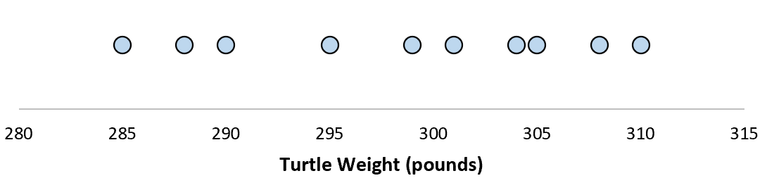
Для этой выборки из 10 черепах мы можем вычислить среднее значение выборки и стандартное отклонение выборки:
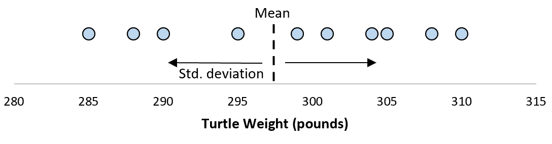
Предположим, что стандартное отклонение оказалось равным 8,68. Это дает нам представление о том, насколько распределен вес этих черепах.
Но предположим, что мы собираем еще одну простую случайную выборку из 10 черепах и также проводим их измерения. Более чем вероятно, что эта выборка из 10 черепах будет иметь немного другое среднее значение и стандартное отклонение, даже если они взяты из одной и той же популяции:
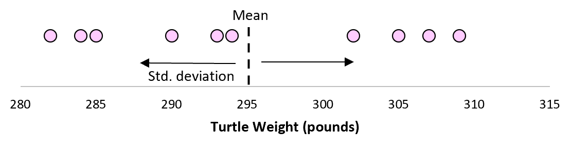
Теперь, если мы представим, что мы берем повторные выборки из одной и той же совокупности и записываем выборочное среднее и выборочное стандартное отклонение для каждой выборки:
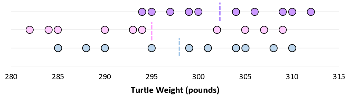
Теперь представьте, что мы наносим каждое среднее значение выборки на одну и ту же строку:

Стандартное отклонение этих средних значений известно как стандартная ошибка.

Формула для фактического расчета стандартной ошибки:
Стандартная ошибка = s/ √n
куда:
- s: стандартное отклонение выборки
- n: размер выборки
Какой смысл использовать стандартную ошибку?
Когда мы вычисляем среднее значение данной выборки, нас на самом деле интересует не среднее значение этой конкретной выборки, а скорее среднее значение большей совокупности, из которой взята выборка.
Однако мы используем выборки, потому что для них гораздо проще собирать данные, чем для всего населения. И, конечно же, среднее значение выборки будет варьироваться от выборки к выборке, поэтому мы используем стандартную ошибку среднего значения как способ измерить, насколько точна наша оценка среднего значения.
Вы заметите из формулы для расчета стандартной ошибки, что по мере увеличения размера выборки (n) стандартная ошибка уменьшается:
Стандартная ошибка = s/ √n
Это должно иметь смысл, поскольку большие размеры выборки уменьшают изменчивость и увеличивают вероятность того, что среднее значение нашей выборки ближе к фактическому среднему значению генеральной совокупности.
Когда использовать стандартное отклонение против стандартной ошибки
Если мы просто заинтересованы в измерении того, насколько разбросаны значения в наборе данных, мы можем использовать стандартное отклонение .
Однако, если мы заинтересованы в количественной оценке неопределенности оценки среднего значения, мы можем использовать стандартную ошибку среднего значения .
В зависимости от вашего конкретного сценария и того, чего вы пытаетесь достичь, вы можете использовать либо стандартное отклонение, либо стандартную ошибку.
Что такое Стандартная формула ошибки?
Стандартная ошибка — это ошибка, которая возникает в распределении выборки при выполнении статистического анализа. Это вариант стандартного отклонения, так как оба понятия соответствуют мерам спреда. Высокая стандартная ошибка соответствует более высокому разбросу данных для взятой выборки. Вычисление формулы стандартной ошибки выполняется для выборки. В то же время стандартное отклонение определяет генеральную совокупность.
Оглавление
- Что такое Стандартная формула ошибки?
- Объяснение
- Пример формулы стандартной ошибки
- Калькулятор стандартной ошибки
- Актуальность и использование
- Стандартная формула ошибки в Excel
- Рекомендуемые статьи
Следовательно, стандартная ошибка среднего значения будет выражаться и определяться в соответствии с соотношением, описанным следующим образом:
σ͞x = σ/√n
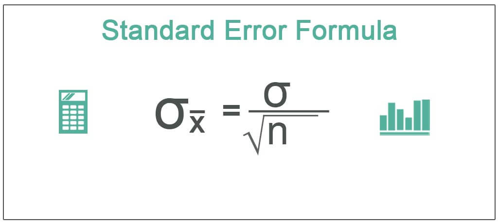
Здесь,
- Стандартная ошибка, выраженная как σ͞x.
- Стандартное отклонение совокупности выражается как σ.
- Количество переменных в выборке, выраженное как n.
В статистическом анализе среднее значение, медиана и мода являются центральной тенденцией. Центральная тенденция Центральная тенденция — это статистическая мера, которая отображает центральную точку всего распределения данных, и вы можете найти ее с помощью 3 различных мер, т. е. среднего, медианы и моды.Подробнее меры. Стандартное отклонение, дисперсия и стандартная ошибка среднего классифицируются как меры изменчивости. Стандартная ошибка среднего для выборочных данных напрямую связана со стандартным отклонением большей совокупности и обратно пропорциональна или связана с квадратным корнем. число. Чтобы использовать эту функцию, введите термин =SQRT и нажмите клавишу табуляции, которая вызовет функцию SQRT. Более того, эта функция принимает один аргумент из нескольких переменных, используемых для создания выборки. Следовательно, если размер выборки Размер выборкиФормула размера выборки отображает соответствующий диапазон генеральной совокупности, в которой проводится эксперимент или опрос. Он измеряется с использованием размера генеральной совокупности, критического значения нормального распределения при требуемом доверительном уровне, доли выборки и предела погрешности. Если больше, то может быть равная вероятность того, что стандартная ошибка также будет большой.
Объяснение
Можно объяснить формулу для стандартной ошибки среднего, используя следующие шаги:
- Определите и организуйте выборку и определите количество переменных.
- Затем среднее значение выборки соответствует количеству переменных, присутствующих в выборке.
- Затем определите стандартное отклонение выборки.
- Затем определите квадратный корень из числа переменных, включенных в выборку.
- Теперь разделите стандартное отклонение, вычисленное на шаге 3, на полученное значение на шаге 4, чтобы получить стандартную ошибку.
Пример формулы стандартной ошибки
Ниже приведены примеры формул для расчета стандартной ошибки.
.free_excel_div{фон:#d9d9d9;размер шрифта:16px;радиус границы:7px;позиция:относительная;margin:30px;padding:25px 25px 25px 45px}.free_excel_div:before{content:»»;фон:url(центр центр без повтора #207245;ширина:70px;высота:70px;позиция:абсолютная;верх:50%;margin-top:-35px;слева:-35px;граница:5px сплошная #fff;граница-радиус:50%} Вы можете скачать этот шаблон стандартной формулы ошибки Excel здесь — Стандартная формула ошибки Шаблон Excel
Пример №1
Возьмем в качестве примера акции ABC. В течение 30 лет акции приносили средний долларовый доход в размере 45 долларов. Кроме того, было замечено, что акции приносят прибыль со стандартным отклонением в 2 доллара. Помогите инвестору рассчитать общую стандартную ошибку средней доходности, предлагаемой акцией ABC.
Решение:
- Стандартное отклонение (σ) = $2
- Количество лет (n) = 30
- Средняя доходность в долларах = 45 долларов.
Расчет стандартной ошибки выглядит следующим образом:

- σ͞x = σ/√n
- = 2 доллара США/√30
- = 2 доллара США / 5,4773
Стандартная ошибка,

- σx = 0,3651 доллара США
Таким образом, инвестиция предлагает инвестору стандартную долларовую ошибку в среднем 0,36515 доллара при удерживании позиции ABC в течение 30 лет. Однако, если бы акции сохранялись для более высокого инвестиционного горизонта, то стандартная ошибка среднего значения в долларах значительно уменьшилась бы.
Пример #2
Возьмем в качестве примера инвестора, который получил следующую доходность акций XYZ:
Год инвестиций Предлагаемая доходность120%225%35%410%
Помогите инвестору рассчитать общую стандартную ошибку средней доходности акций XYZ.
Решение:
Сначала определите среднее значение доходности, как показано ниже: –

- ͞X = (x1+x2+x3+x4)/количество лет
- = (20+25+5+10)/4
- =15%
Теперь определите стандартное отклонение доходности, как показано ниже: –

- σ = √ ((x1-͞X)2 + (x2-͞X)2 + (x3-͞X)2 + (x4-͞X)2) / √ (количество лет -1)
- = √ ((20-15) 2 + (25-15) 2 + (5-15) 2 + (10-15) 2) / √ (4-1)
- = (√ (5) 2 + (10) 2 + (-10) 2 + (-5) 2 ) / √ (3)
- = (√25+100+100+25)/ √ (3)
- =√250/√3
- =√83,3333
- «=» 9,1287%
Теперь вычисление стандартной ошибки выглядит следующим образом:

- σ͞x = σ/√n
- = 9,128709/√4
- = 9,128709/2
Стандартная ошибка,

- σx = 4,56%
Таким образом, инвестиции предлагают инвестору стандартную ошибку в долларах в среднем 4,56% при удержании позиции XYZ в течение 4 лет.
Калькулятор стандартной ошибки
Вы можете использовать следующий калькулятор.
.cal-tbl td{ верхняя граница: 0 !важно; }.cal-tbl tr{ высота строки: 0.5em; } Только экран @media и (минимальная ширина устройства: 320 пикселей) и (максимальная ширина устройства: 480 пикселей) { .cal-tbl tr{ line-height: 1em !important; } } σnСтандартная формула ошибки
Формула стандартной ошибки =σ =√n 0 = 0√0
Актуальность и использование
Стандартная ошибка имеет тенденцию быть высокой, если размер выборки для анализа мал. Следовательно, выборка всегда берется из большей совокупности, которая включает больший размер переменных. Это всегда помогает статистику определить достоверность среднего значения выборки относительно среднего значения генеральной совокупности.
Большая стандартная ошибка говорит статистику, что выборка неоднородна в отношении среднего значения генеральной совокупности. Относительно населения наблюдается большой разброс в выборке. Точно так же небольшая стандартная ошибка говорит статистику, что выборка однородна относительно среднего значения генеральной совокупности. Отсутствуют или незначительные различия в выборке относительно населения.
Не следует смешивать его со стандартным отклонением. Вместо этого следует рассчитать стандартное отклонение для всей совокупности. Стандартная ошибкаСтандартная ошибкаСтандартная ошибка (SE) — это метрика, которая измеряет точность выборочного распределения, обозначающего совокупность, с использованием стандартного отклонения. Другими словами, это мера дисперсии среднего значения выборки, связанная со средним значением генеральной совокупности, а не стандартное отклонение. С другой стороны, оно определяется для среднего значения выборки.
Стандартная формула ошибки в Excel
Теперь давайте возьмем пример Excel, чтобы проиллюстрировать концепцию стандартной формулы ошибки в шаблоне Excel ниже. Предположим, администрация школы хочет определить стандартную ошибку среднего значения роста футболистов.
Выборка состоит из следующих значений: –

Помогите администрации оценить стандартную ошибку среднего значения.
Шаг 1: Определите среднее значение, как показано ниже: –
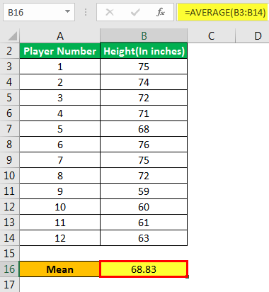
Шаг 2: Определите стандартное отклонение, как показано ниже: –

Шаг 3: Определите стандартную ошибку среднего значения, как показано ниже: –

Следовательно, стандартная ошибка среднего значения для футболистов составляет 1,846 дюйма. Руководство должно заметить, что оно значительно велико. Таким образом, выборочные данные, взятые для анализа, неоднородны и имеют большую дисперсию.
Руководству следует либо исключить более мелких игроков, либо добавить игроков значительно выше, чтобы сбалансировать средний рост футбольной команды, заменив их людьми с меньшим ростом по сравнению с их сверстниками.
Рекомендуемые статьи
Эта статья была руководством по формуле стандартной ошибки. Здесь мы обсуждаем формулу для расчета среднего значения, стандартную ошибку, примеры и загружаемый лист Excel. Вы можете узнать больше из следующих статей: –
- Формула рентабельности EBITDA
- Формула валовой прибыли
- Формула относительного стандартного отклонения
- Формула погрешности