Pandas матрица ошибок

In this short tutorial, you’ll see a full example of a Confusion Matrix in Python.

Topics to be reviewed:

• Creating a Confusion Matrix using pandas
• Displaying the Confusion Matrix using seaborn
• Getting additional stats via pandas_ml
• Working with non-numeric data

Creating a Confusion Matrix in Python using Pandas

To start, here is the dataset to be used for the Confusion Matrix in Python:

y_actual	y_predicted
1	1
0	1
0	0
1	1
0	0
1	1
0	1
0	0
1	1
0	0
1	0
0	0

You can then capture this data in Python by creating pandas DataFrame using this code:

import pandas as pd

data = {'y_actual':    [1, 0, 0, 1, 0, 1, 0, 0, 1, 0, 1, 0],
        'y_predicted': [1, 1, 0, 1, 0, 1, 1, 0, 1, 0, 0, 0]
        }

df = pd.DataFrame(data)
print(df)

This is how the data would look like once you run the code:

    y_actual  y_predicted
0          1            1
1          0            1
2          0            0
3          1            1
4          0            0
5          1            1
6          0            1
7          0            0
8          1            1
9          0            0
10         1            0
11         0            0

To create the Confusion Matrix using pandas, you’ll need to apply the pd.crosstab as follows:

confusion_matrix = pd.crosstab(df['y_actual'], df['y_predicted'], rownames=['Actual'], colnames=['Predicted'])
print (confusion_matrix)

And here is the full Python code to create the Confusion Matrix:

import pandas as pd

data = {'y_actual':    [1, 0, 0, 1, 0, 1, 0, 0, 1, 0, 1, 0],
        'y_predicted': [1, 1, 0, 1, 0, 1, 1, 0, 1, 0, 0, 0]
        }

df = pd.DataFrame(data)

confusion_matrix = pd.crosstab(df['y_actual'], df['y_predicted'], rownames=['Actual'], colnames=['Predicted'])
print(confusion_matrix)

Run the code and you’ll get the following matrix:

Predicted  0  1
Actual         
0          5  2
1          1  4

Displaying the Confusion Matrix using seaborn

The matrix you just created in the previous section was rather basic.

You can use the seaborn package in Python to get a more vivid display of the matrix. To accomplish this task, you’ll need to add the following two components into the code:

• import seaborn as sn
• sn.heatmap(confusion_matrix, annot=True)

You’ll also need to use the matplotlib package to plot the results by adding:

• import matplotlib.pyplot as plt
• plt.show()

Putting everything together:

import pandas as pd
import seaborn as sn
import matplotlib.pyplot as plt

data = {'y_actual':    [1, 0, 0, 1, 0, 1, 0, 0, 1, 0, 1, 0],
        'y_predicted': [1, 1, 0, 1, 0, 1, 1, 0, 1, 0, 0, 0]
        }

df = pd.DataFrame(data)
confusion_matrix = pd.crosstab(df['y_actual'], df['y_predicted'], rownames=['Actual'], colnames=['Predicted'])

sn.heatmap(confusion_matrix, annot=True)
plt.show()

Optionally, you can also add the totals at the margins of the confusion matrix by setting margins=True.

So your Python code would look like this:

import pandas as pd
import seaborn as sn
import matplotlib.pyplot as plt

data = {'y_actual':    [1, 0, 0, 1, 0, 1, 0, 0, 1, 0, 1, 0],
        'y_predicted': [1, 1, 0, 1, 0, 1, 1, 0, 1, 0, 0, 0]
        }

df = pd.DataFrame(data)
confusion_matrix = pd.crosstab(df['y_actual'], df['y_predicted'], rownames=['Actual'], colnames=['Predicted'], margins=True)

sn.heatmap(confusion_matrix, annot=True)
plt.show()

Getting additional stats using pandas_ml

You may print additional stats (such as the Accuracy) using the pandas_ml package in Python. You can install the pandas_ml package using PIP:

pip install pandas_ml

You’ll then need to add the following syntax into the code:

confusion_matrix = ConfusionMatrix(df['y_actual'], df['y_predicted'])
confusion_matrix.print_stats()

Here is the complete code that you can use to get the additional stats:

import pandas as pd
from pandas_ml import ConfusionMatrix

data = {'y_actual':    [1, 0, 0, 1, 0, 1, 0, 0, 1, 0, 1, 0],
        'y_predicted': [1, 1, 0, 1, 0, 1, 1, 0, 1, 0, 0, 0]
        }

df = pd.DataFrame(data)
confusion_matrix = ConfusionMatrix(df['y_actual'], df['y_predicted'])
confusion_matrix.print_stats()

Run the code, and you’ll see the measurements below (note that if you’re getting an error when running the code, you may consider changing the version of pandas. For example, you may change the version of pandas to 0.23.4 using this command: pip install pandas==0.23.4):

population: 12
P: 5
N: 7
PositiveTest: 6
NegativeTest: 6
TP: 4
TN: 5
FP: 2
FN: 1
ACC: 0.75

For our example:

• TP = True Positives = 4
• TN = True Negatives = 5
• FP = False Positives = 2
• FN = False Negatives = 1

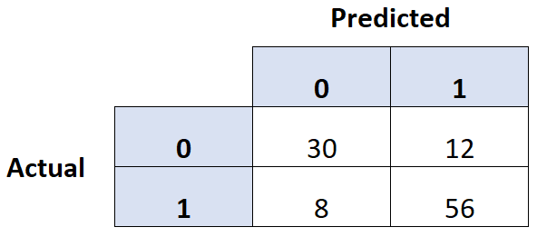
You can also observe the TP, TN, FP and FN directly from the Confusion Matrix:

For a population of 12, the Accuracy is:

Accuracy = (TP+TN)/population = (4+5)/12 = 0.75

Working with non-numeric data

So far you have seen how to create a Confusion Matrix using numeric data. But what if your data is non-numeric?

For example, what if your data contained non-numeric values, such as ‘Yes’ and ‘No’ (rather than ‘1’ and ‘0’)?

In this case:

• Yes = 1
• No = 0

So the dataset would look like this:

y_actual	y_predicted
Yes	Yes
No	Yes
No	No
Yes	Yes
No	No
Yes	Yes
No	Yes
No	No
Yes	Yes
No	No
Yes	No
No	No

You can then apply a simple mapping exercise to map ‘Yes’ to 1, and ‘No’ to 0.

Specifically, you’ll need to add the following portion to the code:

df['y_actual'] = df['y_actual'].map({'Yes': 1, 'No': 0})
df['y_predicted'] = df['y_predicted'].map({'Yes': 1, 'No': 0})

And this is how the complete Python code would look like:

import pandas as pd
from pandas_ml import ConfusionMatrix

data = {'y_actual':    ['Yes', 'No',  'No', 'Yes', 'No', 'Yes', 'No',  'No', 'Yes', 'No', 'Yes', 'No'],
        'y_predicted': ['Yes', 'Yes', 'No', 'Yes', 'No', 'Yes', 'Yes', 'No', 'Yes', 'No', 'No',  'No']    
        }

df = pd.DataFrame(data)
df['y_actual'] = df['y_actual'].map({'Yes': 1, 'No': 0})
df['y_predicted'] = df['y_predicted'].map({'Yes': 1, 'No': 0})

confusion_matrix = ConfusionMatrix(df['y_actual'], df['y_predicted'])
confusion_matrix.print_stats()

You would then get the same stats:

population: 12
P: 5
N: 7
PositiveTest: 6
NegativeTest: 6
TP: 4
TN: 5
FP: 2
FN: 1
ACC: 0.75

A Dependency Free Multiclass Confusion Matrix

# A Simple Confusion Matrix Implementation
def confusionmatrix(actual, predicted, normalize = False):
    """
    Generate a confusion matrix for multiple classification
    @params:
        actual      - a list of integers or strings for known classes
        predicted   - a list of integers or strings for predicted classes
        normalize   - optional boolean for matrix normalization
    @return:
        matrix      - a 2-dimensional list of pairwise counts
    """
    unique = sorted(set(actual))
    matrix = [[0 for _ in unique] for _ in unique]
    imap   = {key: i for i, key in enumerate(unique)}
    # Generate Confusion Matrix
    for p, a in zip(predicted, actual):
        matrix[imap[p]][imap[a]] += 1
    # Matrix Normalization
    if normalize:
        sigma = sum([sum(matrix[imap[i]]) for i in unique])
        matrix = [row for row in map(lambda i: list(map(lambda j: j / sigma, i)), matrix)]
    return matrix

The approach here is to pair up the unique classes found in the actual vector into a 2-dimensional list. From there, we simply iterate through the zipped actual and predicted vectors and populate the counts using the indices to access the matrix positions.

Usage

cm = confusionmatrix(
    [1, 1, 2, 0, 1, 1, 2, 0, 0, 1], # actual
    [0, 1, 1, 0, 2, 1, 2, 2, 0, 2]  # predicted
)

# And The Output
print(cm)
[[2, 1, 0], [0, 2, 1], [1, 2, 1]]

Note: the actual classes are along the columns and the predicted classes are along the rows.

# Actual
# 0  1  2
  #  #  #   
[[2, 1, 0], # 0
 [0, 2, 1], # 1  Predicted
 [1, 2, 1]] # 2

Class Names Can be Strings or Integers

cm = confusionmatrix(
    ["B", "B", "C", "A", "B", "B", "C", "A", "A", "B"], # actual
    ["A", "B", "B", "A", "C", "B", "C", "C", "A", "C"]  # predicted
)

# And The Output
print(cm)
[[2, 1, 0], [0, 2, 1], [1, 2, 1]]

You Can Also Return The Matrix With Proportions (Normalization)

cm = confusionmatrix(
    ["B", "B", "C", "A", "B", "B", "C", "A", "A", "B"], # actual
    ["A", "B", "B", "A", "C", "B", "C", "C", "A", "C"], # predicted
    normalize = True
)

# And The Output
print(cm)
[[0.2, 0.1, 0.0], [0.0, 0.2, 0.1], [0.1, 0.2, 0.1]]

A More Robust Solution

Since writing this post, I’ve updated my library implementation to be a class that uses a confusion matrix representation internally to compute statistics, in addition to pretty printing the confusion matrix itself. See this Gist.

Example Usage

# Actual & Predicted Classes
actual      = ["A", "B", "C", "C", "B", "C", "C", "B", "A", "A", "B", "A", "B", "C", "A", "B", "C"]
predicted   = ["A", "B", "B", "C", "A", "C", "A", "B", "C", "A", "B", "B", "B", "C", "A", "A", "C"]

# Initialize Performance Class
performance = Performance(actual, predicted)

# Print Confusion Matrix
performance.tabulate()

With the output:

===================================
        Aᴬ      Bᴬ      Cᴬ

Aᴾ      3       2       1

Bᴾ      1       4       1

Cᴾ      1       0       4

Note: classᴾ = Predicted, classᴬ = Actual
===================================

And for the normalized matrix:

# Print Normalized Confusion Matrix
performance.tabulate(normalized = True)

With the normalized output:

===================================
        Aᴬ      Bᴬ      Cᴬ

Aᴾ      17.65%  11.76%  5.88%

Bᴾ      5.88%   23.53%  5.88%

Cᴾ      5.88%   0.00%   23.53%

Note: classᴾ = Predicted, classᴬ = Actual
===================================

• 

from sklearn import metrics
metrics. confusion_matrix (y_actual, y_predicted)

#define array of actual values
y_actual = [0, 0, 0, 0, 0, 0, 0, 0, 0, 0, 1, 1, 1, 1, 1, 1, 1, 1, 1, 1]

#define array of predicted values
y_predicted = [0, 0, 1, 0, 0, 1, 1, 0, 0, 1, 0, 0, 1, 1, 1, 1, 1, 1, 1, 1]

from sklearn import metrics

#create confusion matrix
c_matrix = metrics. confusion_matrix (y_actual, y_predicted)

#print confusion matrix
print(c_matrix)

[[6 4]
 [2 8]]

import pandas as pd

y_actual = pd.Series (y_actual, name='Actual')
y_predicted = pd.Series (y_predicted, name='Predicted')

#create confusion matrix
print(pd.crosstab (y_actual, y_predicted))

Predicted 0 1
Actual 
0 6 4
1 2 8

#print accuracy of model
print(metrics. accuracy_score (y_actual, y_predicted))

0.7

#print precision value of model
print(metrics. precision_score (y_actual, y_predicted))

0.667

#print recall value of model
print(metrics. recall_score (y_actual, y_predicted))

0.8

Опубликовано вт, 02/09/2021 — 15:05 пользователем Ksenia