
In the error correction model (ECM) introduced by Granger, Newbold (1974) and Yule (1936), the data being analyzed has a long-term stochastic trend known as cointegration. Error correction expresses that deviations or errors from long-term equilibrium affect short-term dynamics. If the economic time series contains unit roots, the time series is unsteady. Two unsteady and unrelated time series may show a significant relationship when using the least squares method in regression analysis. The error correction model analyzes the effects between long-term and short-term time series data and predicts the time it takes for the dependent variable to return to equilibrium, but the Engel-Granger method has many problems. Johansen has announced a vector error correction model (VECM) to solve the problem. VECM is an error correction model with the concept of a vector autoregressive model (VAR), which is one of the multiple time series models that assume bidirectional causality. Therefore, the vector error correction model is also one of the multiple time series models.
ECM (Wiki simple translation)
An error correction model (ECM) is a multiple time series model in which multiple underlying variables are used for data with long-term stochastic trends called cointegrations. ECM helps estimate the short-term and long-term effects of one time series on another, and is theoretically supported. The error correction captures the fact that the early error from the long-term equilibrium affects the short-term dynamics. Therefore, ECM can directly estimate the rate at which the dependent variable returns to equilibrium after changes in other variables.
history
Yule (1936) and Granger and Newbold (1974) first focused on the problem of fake correlation and found a solution in time series analysis. In two completely unrelated sum (non-stationary) processes, one tends to show a statistically significant relationship with respect to the other by regression analysis. Therefore, it can be mistaken that there is a true relationship between these variables. The usual least squares method is inconsistent and commonly used test statistics are not valid. In particular, Monte Carlo simulations have shown that very high $ R ^ 2 $, individually very high t-statistics, and low Durbin-Watson statistics are obtained. Technically speaking, Phillips (1986) proves that as the sample size increases, the parameter estimates do not stochastically converge, the intercept diverges, and the gradient becomes a non-degenerate distribution. However, because it reflects the long-term relationships between these variables, it is possible that there is a common stochastic trend in both time series that the researcher is really interested in.
Due to the stochastic nature of the trend, the integration process cannot be divided into a deterministic (predictable) trend and a stationary time series containing deviations from the trend. Even a random walk with the deterministic trend removed will eventually show a fake correlation. Therefore, trend removal does not solve the estimation problem. In the Box-Jenkins method, in many time series (economics, etc.), it is generally considered that the first-order difference is steady, and the difference of the time series data is taken to estimate a model such as ARIMA. Forecasts from such models reflect the periodicity and seasonality of the data, however, the long-term adjustment information of the level (original series, price) is lost and the long-term forecasts become unreliable. As a result, Sargan (1964) developed an ECM methodology that retains the information contained in the level.
Estimate
Several methods are known for estimating the sophisticated dynamic model as described above. Among these are the Engle and Granger two-step approach and the vector-based VECM using Johansen’s method of estimating ECM in one step.
Engle and Granger’s two-step approach
The first step is to test in advance whether the individual time series used are non-stationary. Use the standard unit root DF and ADF tests (to solve the problem of series correlation error). Consider the case of two different time series $ x_ {t} $ and $ y_ {t} $. If both are I (0), standard regression analysis is valid. For sums of different orders, for example, if one is I (1) and the other is I (0), then the model needs to be transformed. If both are sums of the same order (usually I (1)), then an ECM model of the form can be estimated:
A(L)Delta y_{t}=gamma +B(L)Delta x_{t}+alpha (y_{t-1}-beta_{0}-beta_{1}x_{t-1})+nu_{t}
If both are cointegrations and this ECM exists, they are said to be cointegrations by the Engle–Granger representation theorem. Next, we estimate the model $ y_ {t} = beta_ {0} + beta_ {1} x_ {t} + varepsilon_ {t} $ using the usual least squares method. If the regression is not masquerading as determined by the test criteria above, not only is the usual least squares valid, but it is actually super-matching (Stock, 1987). Then save the predicted residuals $ hat { varepsilon_ {t}} = y_ {t}- beta_ {0}- beta_ {1} x_ {t} $ from this regression, and the diff variable and delay Used for regression of error term.
A(L)Delta y_{t}=gamma +B(L)Delta x_{t}+alpha {hat {varepsilon }}_{t-1}+nu _{t}
Then test the cointegration using the standard t-statistic of $ alpha $. This method is easy, but it has a number of problems.
-The statistical detection power of the univariate unit root test used in the first stage is low.
—The selection of the dependent variable in the first stage affects the test result. That is, $ x_ {t} $, determined by Granger’s causality, has weak exogenous properties.
—May have a potentially small sample bias.
-The $ alpha $ cointegration test does not follow the standard distribution.
—The distribution of the OLS estimator of the cointegration vector is very complicated and not normally distributed. Therefore, the validity of the long-term parameters in the first regression of obtaining the residuals cannot be verified.
—Only one cointegration relationship can be examined.
VECM
The Engle-Granger approach described above has many weaknesses. That is, one variable is restricted to only a single equation designated as the dependent variable. This variable is explained by another variable that is supposed to be weakly exogenous to the parameter of interest. Also, check whether the time series is I (0) or I (1) by pretest. These weaknesses can be addressed by Johansen’s method. The advantage is that no pretests are required, there is no problem with a large number of cointegration relationships, all are treated as endogenous variables, and tests related to long-term parameters are possible. As a result, the model adds error correction capabilities to the exogenous model known as vector autoregressive (VAR) and is known as the vector error correction model (VECM). The procedure is as follows.
Step 1: Estimate an unconstrained VAR that may contain transient variables
Step 2: Cointegration test using Johansen’s test
Step 3: Create and analyze VECM.
ECM example
The idea of cointegration can be shown by a simple macroeconomic example. It is assumed that consumption $ C_ {t} $ and disposable income $ Y_ {t} $ are macroeconomic time series with long-term relationships. Specifically, the average consumption tendency is set to 90%. In other words, $ C_ {t} = 0.9Y_ {t} $ holds in the long run. From the econometric point of view, the error from regression $ varepsilon_ {t} (= C_ {t}- beta Y_ {t}) $ is the steady time series, $ Y_ {t} $ and $ C_ {t} If $ is non-stationary, then this long-term relationship (also known as cointegration) exists. Also, if $ Y_ {t} $ suddenly changes by $ Delta Y_ {t} $, it is assumed that $ C_ {t} $ changes. $ Delta C_ {t} = 0.5 Delta Y_ {t} $, that is, the marginal consumption tendency is 50%. The final assumption is that the gap between current consumption and equilibrium consumption is reduced by 20% over each period.
With this setting, change the consumption level $ Delta C_ {t} = C_ {t} —C_ {t-1} $ to $ Delta C_ {t} = 0.5 Delta Y_ {t} -0.2 (C_ {t) -1} -0.9Y_ {t-1}) + varepsilon_ {t} $.
The first term of RHS explains the short-term effect of changes in $ Y_ {t} $ on $ C_ {t} $, the second term explains the long-term relationship of variables towards equilibrium, and the third. The term reflects a random shock to the system, such as a shock of consumer confidence that affects consumption.
To see how the model works, consider two types of shocks, permanent and temporary. For simplicity, zero $ varepsilon_ {t} $ for every t.
Suppose the system is in equilibrium for period t − 1. That is, $ C_ {t-1} = 0.9Y_ {t-1} $.
Suppose $ Y_ {t} $ increases by 10 in period t, but then returns to the previous level. In that case, $ C_ {t} $ increases by 5 (half of 10) at the beginning (period t), but in the second and subsequent periods, $ C_ {t} $ begins to decrease and converges to the initial level.
In contrast, if the impact on $ Y_ {t} $ is permanent, $ C_ {t} $ slowly converges to a value greater than 9 above the initial $ C_ {{t-1}} $.
Before learning the vector error correction model
Basic knowledge (Simplified partial translation of 1.2 in [1])
We think that the value of a specific economic variable is the realization value of a random variable for a specific period, and the time series is generated by a stochastic process. To clarify the basic concept, let’s take a quick look at some basic definitions and expressions.
Ω is a set of all basic events (sample space), and (Ω, F, Pr) is a probability space. F is the sigma algebra of the event, or the complement of Ω, and Pr is the probability measure defined by F. The random variable y is a real-valued function $ A_c $ = {ω ∈ Ω | y (ω) ≤ c} ∈ F defined by Ω for each real number c, and $ A_c $ has a probability defined by Pr. It is an event to be done. The function F: R → [0, 1] is defined by $ F (c) = Pr (A_c) $ and is a distribution function of $ y $.
The K-dimensional random vector or the random variable K-dimensional vector is a function from Ω to y in the K-dimensional Euclidean space $ R ^ K $. That is, y maps $ y (ω) = (y_1 (ω), …, y_K (ω)) ^ prime $ to ω ∈ Ω, respectively, $ c = (c_1, …, c_K ) ∈ R_K $, $ A_c = {ω | y_1 (ω) ≤ c_1, cdots, y_K (ω) ≤ c_K} ∈ F $. Function F: RK → [0,1] is defined by $ F (c) = Pr (A_c) $ and is a joint distribution of y functions.
Suppose Z is a set of subscripts with up to countless elements, eg, a set of all integers or all positive integers. The (discrete) stochastic process is a real-valued function of y: Z × Ω → R, which is determined every t ∈ Z, and y (t, ω) is a random variable. The random variable corresponding to t is shown as $ y_t $, and the underlying probability space is not mentioned. In that case, we consider that all members $ y_t $ of the stochastic process are defined in the same probability space. Usually, if the meaning of a symbol is clear from the context, the stochastic process is also indicated by $ y_t $.
The stochastic process is described as a joint distribution function of all finite subsets of $ y_t $ when t ∈ S ⊂ Z. In practice, the complete system of distribution is often unknown, so we often use the first and second moments of the distribution. That is, we use the mean $ E (y_t) = mu_t $, the variance $ E [y_t- mu_t ^ 2] $, and the covariance $ E [(y_t- mu_t) (y_s- mu_s)] $.
The K-dimensional vector stochastic process or multivariate stochastic process is a function of y: Z × Ω → $ R ^ K $, and for each determined t ∈ Z, y (t, ω) is a K-dimensional probability vector. .. Use $ y_t $ for the probability vector corresponding to the determined t ∈ Z. Also, the complete stochastic process may be represented by $ y_t $. This particular meaning becomes clear from the context. The stochastic properties are the same as in the univariate process. That is, the stochastic properties are summarized as a joint distribution function of all finite complement families of the probability vector $ y_t $. In practice, first-order and second-order moments derived from all related random variables are used.
The realization of the (vector) stochastic process is the (vector) sequence set $ y_t ( omega) $ for ω fixed by t ∈ Z. In other words, the realization value of the stochastic process is the function Z → $ R ^ K $ of t → $ y_t $ (ω). Time series (s) are considered such realizations or, in some cases, finite parts of such realizations. That is, for example, it is composed of (vector) $ y_1 ( omega), dots, y_T ( omega) $. The underlying stochastic process is thought to have generated the time series (s) and is called the time series generation or generation process, or data generation process (DGP). The time series $ y_1 ( omega), cdots, y_T ( omega) $ is usually indicated by $ y_1, cdots, y_T $, or simply the underlying stochastic process $ y_t $ if there is no confusion. Is done. The number T of observations is called the sample size or the length of the time series.
VAR process (simplified partial translation of 1.3 in [1])
Since linear functions are easy to handle, we start by predicting past observations with linear functions. Consider the univariate time series $ y_t $ and $ h = 1 $ future forecast. If f (・) is a linear function,
hat{y_{T+1}}=nu+alpha_1 y_T+alpha_2 y_{T-1}+cdots
Will be. The prediction formula uses the past value y of a finite number p,
hat{y_{T+1}} = nu + alpha_1y_{T}+alpha_2y_{T-1} +cdots+alpha_p y_{T-p} + 1
Will be. Of course, the true value $ y_ {T +1} $ and the predicted $ hat {y_ {T +1}} $ are not exactly the same, so
If the prediction error is $ u_ {T +1} = hat {y_ {T +1}} − y_ {T +1} $
y_{T +1} = y_{ T +1} + u_{T +1} =nu + alpha_1 y_T+cdots+alpha_p y_{T-p + 1} + u_{T +1}
Will be. Here, assuming that the numerical value is the realization value of the random variable, the autoregressive process is used for data generation.
y_t =nu + alpha_1 y{t−1} +cdots+ alpha_p y_{t−p} + u_t
Is applied in each period T. Here, $ y_t $, $ y_ {t−1}, cdots, y_ {t−p} $, and $ u_t $ are random variables. In the autoregressive (AR) process, we assume that the prediction errors $ u_t $ in different periods are uncorrelated, that is, $ u_t $ and $ u_s $ are uncorrelated at $ s = t $. That is, since all useful past information $ y_t $ is used for prediction, there is no systematic prediction error.
Considering multiple time series, first
hat{y_{k,T +1}} =nu + alpha_{k1,1}y_{1,T} +alpha_{k2,1}y_{2,T} +
cdots+alpha_{kK,1}y_{K,T}+cdots+alpha_{k1,p}y_{1,T-p+1} +cdots+alpha_{kK,p}y_{K,T-p+1}
It is natural to extend $ k = 1, cdots K $.
To simplify the notation, $ y_t = (y_ {1t}, cdots, y_ {Kt}), hat {y_t}: = ( hat {y_ {1t}}, cdots, hat {y_ {Kt}}), nu = ( nu_1, cdots, nu_K) $ and
A_i=| matrix |(Abbreviation)|
Then, the above vector equation can be described compactly as follows.
y_{T+1}=nu+ A_1y_T +cdots+ A_py_{T −p + 1}
Since $ y_t $ is a vector of random variables, this predictor is the best prediction obtained from a vector autoregressive model of the form:
y_t =nu+ A1y_{t−1} +cdots+ A_py_{t−p} + u_t
Here, $ u_t = (u_ {1t}, cdots, u_ {Kt}) $ is a continuous time series of K-order probability vectors in which the mean of the vectors is zero and is distributed independently and uniformly.
VAR (p) Stabilization process (simplified partial translation of 2.1.1 of [1])
VAR (p) model (VAR model of degree p)
y_t =nu + A_1y_{t−1} +cdots+ A_py_{t−p} + u_t、t = 0、±1、±2、…、(2.1.1)
think about. $ y_t = (y_ {1t}, cdots, y_ {Kt}) ^ prime $ is a random variable (K × 1) vector, $ A_i $ is fixed by a (K × K) coefficient matrix, and $ nu = ( nu_1, cdots, nu_K) ^ prime $ is fixed by the (K × K) coefficient matrix and has a section that can be a non-zero mean $ E (y_t) $. Therefore, $ u_t = (u_ {1t}, cdots, u_ {Kt}) ^ prime $ is K-dimensional white noise or an innovation process. That is, $ s net $, $ E (u_t) = 0, E (u_tu_t ^ prime) = sum_u, E (u_tu_s ^ prime) = 0 $. Unless otherwise stated, the covariance matrix Σu is a non-singular matrix.
Let us consider the process of (2.1.1) a little more. To understand the meaning of the model, consider the VAR (1) model.
y_t =nu + A_1y_{t−1} + u_t cdots (2.1.2)
If this generation mechanism is repeated from $ t = 1 $
y_1 =nu + A_1y_0 + u_1
y_2 =nu+ A_1y_1 + u_2 =nu+ A_1(nu+ A_1y_0 + u_1)+ u_2
=(IK + A_1)nu + A_1^2y_0 + A_1u_1 + u_2
vdots (2.1.3)
y_t =(I_K + A_1 +cdots+ A_1^{t-1})nu+ A^t_1y_0 + sum_{t=0}^{t−1} A_1^iu_{t−i}
vdots
Therefore, the vector $ y_1, cdots, y_t $ is uniquely determined by $ y_0, u_1, cdots, u_t $. The joint distribution of $ y_1, cdots, y_t $ is determined by the joint distribution of $ y_0, u_1, cdots, u_t $.
Sometimes it is assumed that the process starts at a specific period, but sometimes it is more convenient to start from an infinite past. In reality, (2.1.1) corresponds to this. If so, what is the process consistent with the mechanism in (2.1.1)? To consider this problem, reconsider the VAR (1) process in (2.1.2). From (2.1.3)
y_t =nu+ A_1y_t−1 + u_t
=(I_K + A_1 +cdots+ A_j^1)nu+ A_1^{j + 1} y_{t−j−1} +sum_{i=0}^j A_1^i u_{t-i}
If the coefficients of all eigenvalues of $ A_1 $ are less than 1, then the process of $ A ^ i_1 $, $ i = 0,1, cdots $, can be added absolutely. Therefore, infinite sum
sum_{i=1}^infty A=1^j u_{t−i}
Has a root mean square. Also,
(I_K + A_1 +cdots+ A_1^j)nu− rightarrow_{j→infty}(I_K − A_1)^{−1}nu
Furthermore, $ A_1 ^ {j + 1} $ rapidly converges to zero as $ j → infinity $, so the term $ A_1 ^ {j + 1} y_ {t−j−1} $ is ignored in the limit. Will be done. Therefore, if the coefficients of all eigenvalues of $ A_1 $ are less than 1, $ y_t $ is the VAR (1) process of (2.1.2) and $ y_t $ is the well-defined stochastic process.
y_t = µ +sum_{t=0}^infty A_1^i u_{t−i}、t = 0,±1,±2,cdots, (2.1.4)
Then, $ µ = (I_K − A_1) ^ {−1} nu $.
The distribution and joint distribution of $ y_t $ are uniquely determined by the distribution of the process of $ u_t $. The first and second moments of the process of $ y_t $ are for all $ t $
E(y_t)= mu (2.1.5)
It can be seen that it is. And
Gamma y(h)= E(y_t −mu)(y_t−h −mu)^prime
= lim_{n→infty}sum_{i=0}^n sum_{i = 0}^n A_1^i E(u_{t-i}u_{t-h-j}^prime)(A_1^j )^prime (2.1.6)
= lim_{ n = 0}^n A_1^{h + i} sum_u A_1^i=sum_{i=0}^infty A_1^{h+i}sum_u A^{iprime}_1、
Because, in the case of $ s net $, $ E (u_tu_s ^ prime) = 0 $, and in all $ t $, $ E (u_t u_t) = sum_u $.
queueA_1The condition that the coefficients of all eigenvalues of are less than 1 is important and VAR(1)The process is called stable. This condition is|z|le1Against
$ det(I_K − A_1z) ne 0 (2.1.7)$
Will be. The process $ y_t $ of t = 0, ± 1, ± 2, … can also be defined if the stability condition (2.1.7) is not met, but it is defined for all t ∈ Z We don’t do that here because we always assume the stability of the process.
Cointegration process, general stochastic trend, and vector error correction model (simplified partial translation of 6.3 of [1])
Is there really an equilibrium among many economic variables, such as household income and spending, and the price of the same commodity in different markets? The target variable is the vector $ y_t = (y_ {1t}, …, y_ {Kt}) ^ prime $, and their long-term equilibrium relationship is $ beta y_t = beta_1y_ {1t} + ··· · + Beta_Ky_ {Kt} = 0) ^ prime $. Here, $ beta = ( beta_1, …, beta_K) ^ prime $. Over time, this relationship may not be met exactly. Let $ z_t $ be a random variable representing the deviation from the equilibrium, and assume that $ beta y_t = z_t $ holds. If the equilibrium is actually established, the variables $ y_t $ are considered to change with each other and $ z_t $ is considered to be stable. However, with this setting, the variable $ y_t $ can wander extensively as a group. It may be driven by a common stochastic trend. In other words, each variable is a sum, and there is a linear combination of variables that is stationary. A sum variable having this characteristic is called a cointegration.
In general, all components of the K-dimensional $ y_t $ process are $ I (d) $, under $ beta = ( beta_1, cdots, beta_K) ^ prime ne 0 $, $ z_t = beta ^ prime If there is a linear combination of y_t $ and $ z_t $ is $ I (d − b) $, then the variable $ y_t $ is the cointegration of degree $ (d, b) $. It is called and is expressed by $ y_t ~ CI (d, b) $. For example, if all the components of $ y_t $ are I (1) and $ beta y_t $ is stationary (I (0)), then $ y_t to CI (1,1) $. The vector $ beta $ is called the cointegration vector. The process composed of variables that are cointegrations is called the cointegration process. This process was introduced by Granger (1981) and Engle & Granger (1987).
To simplify the term, we use a slightly different definition of cointegration. When $ Delta ^ d y_t $ is stable and $ Delta ^ {d−1} y_t $ is not stable, the K-dimensional $ y_t $ process is called the sum of degrees $ d $, which is easily $ y_t ~ I. Write (d) $. The I (d) process of $ y_t $ is a sum with an order smaller than $ d $, and if there is a linear combination $ beta y_t $ of $ beta ne 0 $, it is called a cointegration. This definition is different from that of Engle & Granger (1987) and does not exclude components of $ y_t $ whose sum order is less than d. If $ y_t $ has only one I (d) component and all other components are stable (I (0)), then $ Delta ^ d y_t $ is stable and $ Delta ^ When {d−1} y_t $ is not stable, the vector $ y_t $ becomes I (d) according to the definition. In such a case, the relationship $ beta y_t $ containing only the stationary component is a cointegration relationship in our terminology. Obviously, this aspect of our definition does not match the original idea of considering a special relationship between sum variables with a common stochastic trend as a cointegration, but distinguishes sums of variables of different degrees. The definition is still valid, not because it just simplifies the term. Readers should have a basic idea of cointegration when it comes to interpreting certain relationships.
Obviously, the cointegration vector is not unique. Multiplying by a non-zero constant yields a cointegration vector. Also, there may be various linearly independent cointegration vectors. For example, if your system has four variables, suppose the first two are in long-term equilibrium and the last two are similar. Therefore, there may be a cointegration vector with zeros in the last two positions and zeros in the first two positions. In addition, all four variables may have a cointegration relationship.
Prior to the introduction of the concept of cointegration, very close error-correcting models were discussed in the field of econometrics. Generally, in the error correction model, the change of the variable is regarded as a dissociation from the equilibrium relationship. For example, suppose $ y_ {1t} $ represents the price of an item in one market and $ y_ {2t} $ corresponds to the price of the same item in another market. Furthermore, it is assumed that the equilibrium between the two variables is given by $ y_ {1t} = beta_1 y_ {2t} $ and that the change in $ y_ {1t} $ depends on the deviation from this equilibrium in the period t − 1. To do.
Delta y_{1t} =alpha_1(y_{1,t−1} −beta_1y_{2,t−1})+ u_{1t}
A similar relationship may apply to $ y_ {2t} $
Delta y_{2t} =alpha_2(y_{1t−1} −beta_1y_{2,t−1})+ u_{2t}
In a more general error correction model, $ Delta y_ {it} $ may also depend on previous changes in both variables, for example:
Delta y_{1t} =alpha_1(y_{1,t−1} −beta_1y_{2,t−1})+ gamma_{11,1}Delta y_{1,t−1} + gamma_{12,1}Delta y_{2,t−1} + u_{1t}、
Delta y_{2t} =alpha_2(y_{1,t−1} −beta_1y_{2,t−1})+ gamma_{21,1}Delta y_{1t}−1 + gamma_{22,1}Delta y_{2,t−1} + u_{2t} / / (6.3.1)
It may also contain a lag before $ Delta y_ {it} $.
To see the close relationship between the error correction model and the concept of cointegration, we assume that both $ y_ {1t} $ and $ y_ {2t} $ are I (1) variables. In that case, all terms in (6.3.1), including $ Delta y_ {it} $, are stable. In addition, $ u_ {1t} $ and $ u_ {2t} $ are white noise errors, which are also stable. Unstable terms are not equivalent to stable processes
alpha_i(y_{1,t−1} −beta_1y_{2,t−1})= Delta y_{it} − gamma_{i1,1}Delta y_{1,t−1} − gamma_{i2,1}Delta y_{2,t−1} − u_{it}
Must also be stable. Therefore, if $ alpha_1 = 0 $ or $ alpha_2 = 0 $, $ y_ {1t}- beta_1 y_ {2t} $ is stable and has a cointegration relationship.
Basic knowledge 2 (written with reference to [2] 2.1)
Random walk
X_t=X_{t-1}+varepsilon_t
Can be described as. If you rewrite this
X_t=X_{t-1}+varepsilon_t
X_{t-1}=X_{t-2}+varepsilon_{t-1}
X_{t-2}=X_{t-2}+varepsilon_{t-2}
vdots
X_{2}=X_{1}+varepsilon_{2}
X_{1}=X_{0}+varepsilon_{1}
Can be written. If you add this up, the X diagonally below will be offset, so in the end
X_t=X_0+sum varepsilon_t
Can be described as. Random walk is the sum of random numbers.
Then do the same for AR (1). However, multiply each line by $ C_ {t-j} (= Pi ^ j $) so that the diagonally lower X is offset by the left side.
X_t=Pi X_{t-1}+varepsilon_t
Can be described as. If you rewrite this
X_t=Pi X_{t-1}+varepsilon_t
X_{t-1}=Pi X_{t-2}+varepsilon_{t-1}
X_{t-2}=Pi X_{t-2}+varepsilon_{t-2}
vdots
X_{2}=Pi X_{1}+varepsilon_{2}
X_{1}=Pi X_{0}+varepsilon_{1}
Can be written. If you add this up, the X diagonally below will be offset, so in the end
X_t=C_{t-1} Pi X_0 +sum_{i=0}^{t-1} C_i varepsilon_{t-j}
Can be described as. It is the sum of random numbers again,
X_t=Pi^t X_0 +sum_{i=0}^{t-1} Pi^t varepsilon_{t-j}
So if $ Pi <1 $
X_t^*=sum_{i=0}^{infty}Pi^ivarepsilon_t
Converges to.
Basic knowledge 3 (written with reference to [2] 3.1)
If $ X_t $ is I (1) and A is a full-rank pxp matrix, then $ AX_t $ is also $ I (0) $.
X_t=X_0+sum Y_i
And.
$ Y_t = sum_ {i = 0} ^ infinty C_i varepsilon_ {ti} $ as $ I (0) $ $ sum_ {i = 0} ^ infinty C_i ne 0 $, then $ X_t $ Is non-stationary.
$ C_z = sum_ {i = 0} ^ infinity C_i z ^ i $ as $ C ^ * (z) $
C^{*}=sum_{i=0}^infty frac{C(z)-C(1)}{1-z}=sum_{i=0}^infty C_i^*z^i
Is defined as. Therefore,
X_t=X_0+sum_{i=1}^t Y_i=X_0+Csum_{i=1}^tvarepsilon_i+Y_t^*-Y_0^*
This process is non-stationary because it is $ C ne 0 $ and $ Y_t = Delta X_t $. Multiply both sides by $ beta $
beta^`X_t=beta^`X_0 +beta^`Csum_{i=1}^tvarepsilon_t+beta^` Y_t^*- beta^`Y_0^*
In order for $ beta ^ X_t $ to be steady, $ beta ^ C = 0 $
beta^`X_t=beta^`Y_t^*+beta^`X_0-beta^`Y_0^*
It should be $ beta ^ X_0 = beta ^ Y_0 ^ * $. Then
beta^`X_t=beta^`Y_t^*
Assuming that $ X_t $ is $ I (1) $, if $ beta ^ `X_t $ is stationary, then $ X_t $ is a cointegration.
The induction system of the error correction model
Delta X_t= alpha beta^` X_{t-1}+varepsilon_t
Let $ X_0 $ be the initial value and $ alpha $ and $ beta $ be the p x r matrix. $ beta ^ X_t = E ( beta ^ X_t) = c $ defines the underlying economy. The adjustment coefficient $ alpha $ tries to return the unbalanced error $ beta ^ `X_t-c $ to the correct state.
Basic knowledge 4 (written with reference to [2] 4.1)
X_t=Pi_1 X_{t-1}+varepsilon_t
Subtract $ X_ {t-1} $ from both sides of
X_t-X_{t-1}=Pi_1 X_{t-1} — X_{t-1}+varepsilon_t
Will be. To summarize this
Delta X_t=(Pi_1-I) X_{t-1} +varepsilon_t
Delta X_t=Pi_1 X_{t-1} +varepsilon_t
It becomes the form of an error correction model. Be careful when handling $ Pi $.
This is easier to understand if the lag is secondary.
Delta X_t=Pi_1 X_{t-1} +sum_{i=1}^{k-1} Gamma_i Delta X_{t-1}+varepsilon_t
If the lag is primary, the $ Gamma $ part will drop.
An example of intuitively understanding the meaning of cointegration
Example 3.1 Johansen, S. 1995. Likelihood-Based Inference in Cointegrated Vector Autoregressive Models p.37
#Initialization
%matplotlib inline
import matplotlib.pyplot as plt
from statsmodels.tsa.api import VECM
import statsmodels.api as sm
from statsmodels.tsa.base.datetools import dates_from_str
import pandas as pd
import numpy as np
from numpy import linalg as LA
from statsmodels.tsa.vector_ar.vecm import coint_johansen
from statsmodels.tsa.vector_ar.vecm import select_coint_rank
from statsmodels.tsa.vector_ar.vecm import select_order
Two-dimensional process $ X_t $
X_{1t}=sum_{i=1}t epsilon_{1i}+epsilon_{2t},
X_{2t}=sum_{i=1}t epsilon_{1i}+epsilon_{3t},
If defined as, these are cointegrations under the cointegration vector of $ beta ^ = (a, -1) $. The linear relationship $ beta ^ X_t = aX_ {1t} -X_ {2t} = a epsilon_ {2t}- epsilon_ {3t} $ is stationary, so let’s check it.
Oxford University Press.
n=10000
a=0.3
e1=np.random.normal(0,1,n)#.reshape([n,1])
e2=np.random.normal(0,1,n)#.reshape([n,1])
e3=np.random.normal(0,1,n)#.reshape([n,1])
X1=np.cumsum(e1)+e2
X2=a*np.cumsum(e1)+e3
X=np.concatenate([X1.reshape([n,1]),X2.reshape([n,1])],1)
plt.plot(X)

From the graph, it can be seen that both are in the process of integration, but they behave in the same way.
betaX=a*X1-X2
plt.plot(betaX)

Stationarity can be confirmed. Let’s examine some more characteristics.
from statsmodels.tsa.vector_ar.vecm import coint_johansen
jres = coint_johansen(X, det_order=0, k_ar_diff=2)
print('critical value of max eigen value statistic',jres.cvm)
print('maximum eigenvalue statistic',jres.lr2)
print('critical value of trace statistic',jres.cvt)
print('Trace statistic',jres.lr1)
print('eigen values of VECM coefficient matrix',jres.eig)
print('eigen vectors of VECM coefficient matrix',jres.evec)
print('Order of eigenvalues',jres.ind)
print('meth',jres.meth)
critical value (90%, 95%, 99%) of max eigen value statistic
[[12.2971 14.2639 18.52  ]
 [ 2.7055  3.8415  6.6349]]
maximum eigenvalue statistic
[2855.97930446    4.11317178]
critical value of trace statistic
[[13.4294 15.4943 19.9349]
 [ 2.7055  3.8415  6.6349]]
Trace statistic
[2860.09247624    4.11317178]
eigen values of VECM coefficient matrix
[0.24849967 0.00041136]
eigen vectors of VECM coefficient matrix
[[ 0.50076827 -0.03993806]
 [-1.67011922 -0.01128004]]
Order of eigenvalues [0 1]
meth johansen
Next, let’s find out about the rank.
rres = select_coint_rank(X, det_order=-1, k_ar_diff=2)
rres.summary()
Johansen cointegration test using trace test statistic with 5% significance level
r_0	r_1	test statistic	critical value
0	2	2857.	12.32
1	2	1.584	4.130
Next, let’s examine lag.
rres = select_order(X,maxlags=10)
rres.summary()
VECM Order Selection (* highlights the minimums)
AIC	BIC	FPE	HQIC
0	1.079	1.083	2.942	1.081
1	0.9691	0.9764	2.636	0.9716
2	0.9541	0.9642*	2.596	0.9575
3	0.9528*	0.9658	2.593*	0.9572*
4	0.9528	0.9687	2.593	0.9582
5	0.9535	0.9723	2.595	0.9598
6	0.9539	0.9755	2.596	0.9612
7	0.9546	0.9791	2.598	0.9629
8	0.9550	0.9825	2.599	0.9643
9	0.9556	0.9860	2.600	0.9659
10	0.9556	0.9888	2.600	0.9668
Let’s see the result with the VECM model.
model=VECM(X,k_ar_diff=0,deterministic='na')
res=model.fit()
print(res.summary())
                 Loading coefficients (alpha) for equation y1
==============================================================================
                 coef    std err          z      P>|z|      [0.025      0.975]
------------------------------------------------------------------------------
ec1           -0.0805      0.005    -16.217      0.000      -0.090      -0.071
                 Loading coefficients (alpha) for equation y2
==============================================================================
                 coef    std err          z      P>|z|      [0.025      0.975]
------------------------------------------------------------------------------
ec1            0.2708      0.003     86.592      0.000       0.265       0.277
          Cointegration relations for loading-coefficients-column 1
==============================================================================
                 coef    std err          z      P>|z|      [0.025      0.975]
------------------------------------------------------------------------------
beta.1         1.0000          0          0      0.000       1.000       1.000
beta.2        -3.3342      0.004   -850.887      0.000      -3.342      -3.327
==============================================================================
Next,
Add $ X_ {3t} = epsilon_ {4t} $. In this vector process, there are two cointegration vectors (a, -1,0) and (0,0,1).
n=10000
a=0.3
e1=np.random.normal(0,1,n)#.reshape([n,1])
e2=np.random.normal(0,1,n)#.reshape([n,1])
e3=np.random.normal(0,1,n)#.reshape([n,1])
e4=np.random.normal(0,1,n)#.reshape([n,1])
X1=np.cumsum(e1)+e2
X2=a*np.cumsum(e1)+e3
X3=e4
X=np.concatenate([X1.reshape([n,1]),X2.reshape([n,1]),X3.reshape([n,1])],1)
model=VECM(X,k_ar_diff=0,deterministic='na')
res=model.fit()
print(res.summary())
 Loading coefficients (alpha) for equation y1
==============================================================================
                 coef    std err          z      P>|z|      [0.025      0.975]
------------------------------------------------------------------------------
ec1           -0.0319      0.003    -11.006      0.000      -0.038      -0.026
                 Loading coefficients (alpha) for equation y2
==============================================================================
                 coef    std err          z      P>|z|      [0.025      0.975]
------------------------------------------------------------------------------
ec1            0.0962      0.002     42.596      0.000       0.092       0.101
                 Loading coefficients (alpha) for equation y3
==============================================================================
                 coef    std err          z      P>|z|      [0.025      0.975]
------------------------------------------------------------------------------
ec1           -0.1374      0.002    -71.039      0.000      -0.141      -0.134
          Cointegration relations for loading-coefficients-column 1
==============================================================================
                 coef    std err          z      P>|z|      [0.025      0.975]
------------------------------------------------------------------------------
beta.1         1.0000          0          0      0.000       1.000       1.000
beta.2        -3.3418      0.008   -445.090      0.000      -3.357      -3.327
beta.3         4.7902      0.059     81.021      0.000       4.674       4.906
==============================================================================
Example 3.2 Johansen, S. 1995. Likelihood-Based Inference in Cointegrated Vector Autoregressive Models p.37
Next, let’s look at the quadratic sum I (2).

As for X1, X2, and X3, I’m not sure if it will be really steady, so I’ll actually make random numbers. A, b, and c were adjusted so that the graph was easy to see.
n=1000
a=0.3
e1=np.random.normal(0,1,n)#.reshape([n,1])
e2=np.random.normal(0,1,n)#.reshape([n,1])
e3=np.random.normal(0,1,n)#.reshape([n,1])
e4=np.random.normal(0,1,n)#.reshape([n,1])
cs_e1=np.cumsum(e1)
cs_cs_e1=np.cumsum(cs_e1)
cs_e2=np.cumsum(e2)
X1=cs_cs_e1+cs_e2
a=0.5
b=2
X2=a*cs_cs_e1+b*cs_e2+e3
c=100
X3=c*cs_e2+e4
plt.plot(X1)
plt.plot(X2)
plt.plot(X3)

Next, let’s take the actual difference and check the stationarity.
plt.plot(np.diff(X1))
plt.plot(np.diff(np.diff(X1)))

I understand that the difference on the first floor is not steady, but on the second floor it is steady.
plt.plot(np.diff(X2))
plt.plot(np.diff(np.diff(X2)))

The result here is the same.
plt.plot(np.diff(X3))
plt.plot(np.diff(np.diff(X3)))

Vector Error Correcting Models (VECM) statsmodels Manual
The vector error correction model is used to study the relationship between the permanent stochastic trend (unit root) of the objective variable and its short-term dissociation. VECM is used to model the difference series of vectors and identify and estimate these models under the assumption that there are multiple stochastic trends. VECM ($ k_ {ar} -1) $ is
Delta y_t= Pi y_{t−1} + Gamma_1Delta y_{t−1} +dots + Gamma_{k_{ar}-1}Delta y_{t−k_{ar} + 1} + u_t
Takes the form of. Also, $ Pi = alpha beta ^ $. Since these $ alpha $ and $ beta ^ $ cannot be estimated by the least squares method, the eigenvalues and eigenvectors of $ Pi $ are obtained by maximum likelihood estimation of the error correction model, and $ Pi by the cointegration test. Determine the rank of $ and find the eigenvector corresponding to the eigenvalue. See Chapter 7 of [1]. It is also possible to include deterministic terms such as constant terms and trend terms in $ Pi y_ {t−1} $. See [3].
VECM ($ k_ {ar} -1 $) with a deterministic term

Will be. $ D_ {t-1} ^ infinty $ indicates that there is a deterministic term in the cointegration vector (or constraining the cointegration vector). $ eta $ is the relevant estimator. To pass a deterministic term in the cointegration vector, use the argument exog_coint. In the two special cases of constant terms and linear trends, there is an easier way than using these terms. You can pass each of «ci» and «li» to the argument deterministic. Therefore, for the constant term in the cointegration vector, pass «ci» for the argument deterministic or np.ones (len (data)) to exog_coint. In this case, $ D_ {t-1} ^ infinty = 1 $ for all $ t $.
You can also use deterministic terms outside the cointegration vector. These are defined in $ D_t $ in the above equation with an estimator for the matrix $ C $. These terms are specified by passing them to the argument exog. For constant terms and / or linear trends, the argument deterministic can be used instead. Pass «co» for constant terms and «lo» for linear trends. «o» represents the outside. The following table shows the five cases considered in [2]. The last column shows the string to pass to the deterministic argument of each of these cases.
-
class statsmodels.tsa.vector_ar.vecm.VECM(endog, exog=None, exog_coint=None, dates=None, freq=None, missing=’none’, k_ar_diff=1, coint_rank=1, deterministic=’nc’, seasons=0, first_season=0)
-
Class representing a Vector Error Correction Model (VECM).
—Parameters
endog array-like(nobs_tot x neqs)
Two-dimensional endogenous response variable.
exog: ndarray (nobs_tot x neqs) or None
A deterministic term outside the cointegration vector.
exog_coint: ndarray (nobs_tot x neqs) or None
Deterministic term in the cointegration vector.
date array-like datetime, optional.
See statsmodels.tsa.base.tsa_model.TimeSeriesModel for more information.
freqstr, optional
See statsmodels.tsa.base.tsa_model.TimeSeriesModel for more information.
missing str, option,
See statsmodels.base.model.Model for more information.
k_ar_diff int
The order of the difference in the model. Equal to kar-1 in the above equation.
coint_rank int
The cointegration rank is equal to the rank Π of the matrix and the number of columns of α and β.
deterministic str {«nc»、 «co»、 «ci»、 «lo»、 «li»}
«nc»-no deterministic term
«co»-constant outside the cointegration vector
«ci»-constants in the cointegration vector
«lo»-Linear trend outside the cointegration vector
«li»-Linear trend in cointegration vector
Can be combined (eg «cili» or «colo» for linear trends with constant terms). If you use a constant term, you need to choose whether to limit it to a cointegration relationship (ie «ci») or leave it unlimited (ie «co»). Do not use both “ci” and “co”. The same is true for «li» and «lo» when using linear terms. See note for details.
seasons int, default: 0
The number of periods in the seasonal cycle. 0 means there is no season.
first_season int, default: 0
The season of the first observation.
- VECMResults.predict(steps=5, alpha=None, exog_fc=None, exog_coint_fc=None)[source]
Calculate future values in time series
—Parameters
steps int
Prediction period.
alpha float, 0 < alpha < 1 or None
If None, only point predictions are calculated. For float, the confidence interval is also calculated. In this case, the argument represents the trust level.
exog ndarray (steps x self.exog.shape[1])
If self.exog is not None, pass information about future values of exog from this parameter. The ndarray can be larger in the first dimension. In this case, only the first step row is considered.
- Returns
forecast — ndarray (steps x neqs) or three ndarrays
For point predictions: Each row of the returned ndarray represents a prediction of the neqs variable for a particular time period. The first row (index [0]) is the forecast for the next period and the last row (index [steps-1]) is the steps-periods-ahead- forecast.
References
[1] Lütkepohl, H. 2005. New Introduction to Multiple Time Series Analysis. Springer.
[2] Johansen, S. 1995. Likelihood-Based Inference in Cointegrated * *Vector Autoregressive Models. Oxford University Press.
[3] Johansen, S. and K Jusellus 1990. Likelihood-Based Estimation and Inference on Cointegration with application to the demand for money. 0xford Bullretin of Economics and Statisitics,52,169-210
Before analyzing the actual data
Generating artificial data and using that data to understand the characteristics of the model before analyzing the actual data is the most effective weapon.
So let’s generate two non-stationary time series, $ x $ and $ y $, and analyze them with VECM. At that time, set deterministic =’nc’ and K_ar_diff = 0. This is an attempt to limit the variables of the model to only $ alpha $ and $ beta $. At that time, simple regression of $ x $ and $ y $ is performed to obtain beta, and the error is used to estimate alpha. The number of data is $ n = 10000 $. Enough to converge.
n=10000
y=pd.DataFrame(np.random.normal(0,1,n).reshape([n,1]),columns=['y'])
x=pd.DataFrame(np.random.normal(0,1,n).reshape([n,1]),columns=['x'])
data=pd.concat([y.cumsum(),x.cumsum()],axis=1)
data.columns=['y','x']
model=VECM(data,k_ar_diff=0,deterministic='na')
res=model.fit()
print(res.summary())

xx=sm.add_constant(x.cumsum())
res= sm.OLS(y.cumsum(), xx).fit()
print(res.summary())
 Loading coefficients (alpha) for equation y
==============================================================================
                 coef    std err          z      P>|z|      [0.025      0.975]
------------------------------------------------------------------------------
ec1           -0.0005      0.000     -1.671      0.095      -0.001    8.89e-05
                 Loading coefficients (alpha) for equation x
==============================================================================
                 coef    std err          z      P>|z|      [0.025      0.975]
------------------------------------------------------------------------------
ec1        -3.723e-05      0.000     -0.121      0.904      -0.001       0.001
          Cointegration relations for loading-coefficients-column 1
==============================================================================
                 coef    std err          z      P>|z|      [0.025      0.975]
------------------------------------------------------------------------------
beta.1         1.0000          0          0      0.000       1.000       1.000
beta.2        -0.2731      0.382     -0.716      0.474      -1.021       0.475
==============================================================================
                            OLS Regression Results
==============================================================================
Dep. Variable:                      y   R-squared:                       0.126
Model:                            OLS   Adj. R-squared:                  0.126
Method:                 Least Squares   F-statistic:                     1443.
Date:                Sun, 01 Mar 2020   Prob (F-statistic):          4.92e-295
Time:                        02:27:15   Log-Likelihood:                -43187.
No. Observations:               10000   AIC:                         8.638e+04
Df Residuals:                    9998   BIC:                         8.639e+04
Df Model:                           1
Covariance Type:            nonrobust
==============================================================================
                 coef    std err          t      P>|t|      [0.025      0.975]
------------------------------------------------------------------------------
const        -29.8591      0.210   -142.406      0.000     -30.270     -29.448
x             -0.1572      0.004    -37.984      0.000      -0.165      -0.149
==============================================================================
Omnibus:                      414.693   Durbin-Watson:                   0.003
Prob(Omnibus):                  0.000   Jarque-Bera (JB):              401.515
Skew:                          -0.447   Prob(JB):                     6.49e-88
Kurtosis:                       2.593   Cond. No.                         58.5
==============================================================================
u=res.resid
#x1=pd.concat([x,u],axis=1)
#x1=sm.add_constant(x1)

res= sm.OLS(y, u).fit()
print(res.summary())
 OLS Regression Results
=======================================================================================
Dep. Variable:                      y   R-squared (uncentered):                   0.000
Model:                            OLS   Adj. R-squared (uncentered):             -0.000
Method:                 Least Squares   F-statistic:                             0.2729
Date:                Sun, 01 Mar 2020   Prob (F-statistic):                       0.601
Time:                        02:57:55   Log-Likelihood:                         -14187.
No. Observations:               10000   AIC:                                  2.838e+04
Df Residuals:                    9999   BIC:                                  2.838e+04
Df Model:                           1
Covariance Type:            nonrobust
==============================================================================
                 coef    std err          t      P>|t|      [0.025      0.975]
------------------------------------------------------------------------------
x1             0.0001      0.000      0.522      0.601      -0.000       0.001
==============================================================================
Omnibus:                        0.070   Durbin-Watson:                   2.013
Prob(Omnibus):                  0.966   Jarque-Bera (JB):                0.053
Skew:                          -0.002   Prob(JB):                        0.974
Kurtosis:                       3.011   Cond. No.                         1.00
==============================================================================
By moving this over and over again, you should be able to see the meaning and usage of the model. Don’t forget that the data is a random walk.
Example: US macro data
year Period —1959q1 —2009q3
quarter: quarter— 1-4
realgdp: Real Gross Domestic Product-(Bil. Of chained 2005 USD, seasonally adjusted annual rate)
realcons: Real personal consumption-(Bil. Of chained 2005 USD, seasonally adjusted annual rate)
realinv: Real Private Total Domestic Investment (Bil. Of chained 2005 USD, Seasonally Adjusted Annual Rate)
from statsmodels.tsa.api import VECM
import statsmodels.api as sm
from statsmodels.tsa.base.datetools import dates_from_str
import pandas as pd
import numpy as np

mdata = sm.datasets.macrodata.load_pandas().data
dates = mdata[['year', 'quarter']].astype(int).astype(str)
quarterly = dates["year"] + "Q" + dates["quarter"]

quarterly = dates_from_str(quarterly)
mdata = mdata[['realgdp','realcons','realinv']]
mdata.index = pd.DatetimeIndex(quarterly)
data = np.log(mdata).diff().dropna()

model = VECM(data)

results = model.fit()
print(results.summary())
Det. terms outside the coint. relation & lagged endog. parameters for equation realgdp
===============================================================================
                  coef    std err          z      P>|z|      [0.025      0.975]
-------------------------------------------------------------------------------
L1.realgdp     -0.0101      0.147     -0.068      0.945      -0.298       0.278
L1.realcons    -0.4094      0.133     -3.081      0.002      -0.670      -0.149
L1.realinv      0.0039      0.020      0.197      0.843      -0.035       0.043
Det. terms outside the coint. relation & lagged endog. parameters for equation realcons
===============================================================================
                  coef    std err          z      P>|z|      [0.025      0.975]
-------------------------------------------------------------------------------
L1.realgdp      0.0039      0.140      0.028      0.978      -0.270       0.277
L1.realcons    -0.4813      0.126     -3.818      0.000      -0.728      -0.234
L1.realinv     -0.0083      0.019     -0.443      0.658      -0.045       0.028
Det. terms outside the coint. relation & lagged endog. parameters for equation realinv
===============================================================================
                  coef    std err          z      P>|z|      [0.025      0.975]
-------------------------------------------------------------------------------
L1.realgdp      2.3752      0.825      2.879      0.004       0.758       3.992
L1.realcons    -1.4317      0.745     -1.922      0.055      -2.892       0.028
L1.realinv     -0.3738      0.110     -3.383      0.001      -0.590      -0.157
              Loading coefficients (alpha) for equation realgdp
==============================================================================
                 coef    std err          z      P>|z|      [0.025      0.975]
------------------------------------------------------------------------------
ec1           -1.2524      0.141     -8.875      0.000      -1.529      -0.976
              Loading coefficients (alpha) for equation realcons
==============================================================================
                 coef    std err          z      P>|z|      [0.025      0.975]
------------------------------------------------------------------------------
ec1            0.0673      0.134      0.503      0.615      -0.195       0.330
              Loading coefficients (alpha) for equation realinv
==============================================================================
                 coef    std err          z      P>|z|      [0.025      0.975]
------------------------------------------------------------------------------
ec1           -7.3749      0.791     -9.322      0.000      -8.926      -5.824
          Cointegration relations for loading-coefficients-column 1
==============================================================================
                 coef    std err          z      P>|z|      [0.025      0.975]
------------------------------------------------------------------------------
beta.1         1.0000          0          0      0.000       1.000       1.000
beta.2        -0.9514      0.037    -25.704      0.000      -1.024      -0.879
beta.3        -0.0204      0.010     -1.967      0.049      -0.041   -6.88e-05
==============================================================================
Exchange rate analysis
import matplotlib.pyplot as plt
start="1949/5/16"
fx = web.DataReader("DEXJPUS","fred",start)# usdjpy
rf = web.DataReader("USD12MD156N", 'fred',start)
rd = web.DataReader("JPY12MD156N", 'fred',start)
data=pd.concat([fx,rf,rd],axis=1).ffill().dropna()
data.tail()
	DEXJPUS	USD12MD156N	JPY12MD156N
DATE
2019-12-02	109.09	1.96250	0.10283
2019-12-03	108.53	1.93663	0.10367
2019-12-04	108.87	1.91700	0.10567
2019-12-05	108.69	1.92263	0.09833
2019-12-06	108.66	1.92313	0.10833
model = VECM(data)

results = model.fit()
print(results.summary())
Det. terms outside the coint. relation & lagged endog. parameters for equation DEXJPUS
==================================================================================
                     coef    std err          z      P>|z|      [0.025      0.975]
----------------------------------------------------------------------------------
L1.DEXJPUS         0.0179      0.011      1.681      0.093      -0.003       0.039
L1.USD12MD156N     0.2679      0.155      1.729      0.084      -0.036       0.572
L1.JPY12MD156N    -0.1119      0.272     -0.412      0.681      -0.645       0.421
Det. terms outside the coint. relation & lagged endog. parameters for equation USD12MD156N
==================================================================================
                     coef    std err          z      P>|z|      [0.025      0.975]
----------------------------------------------------------------------------------
L1.DEXJPUS         0.0042      0.001      5.762      0.000       0.003       0.006
L1.USD12MD156N     0.0529      0.011      4.931      0.000       0.032       0.074
L1.JPY12MD156N     0.0111      0.019      0.590      0.555      -0.026       0.048
Det. terms outside the coint. relation & lagged endog. parameters for equation JPY12MD156N
==================================================================================
                     coef    std err          z      P>|z|      [0.025      0.975]
----------------------------------------------------------------------------------
L1.DEXJPUS         0.0041      0.000      9.923      0.000       0.003       0.005
L1.USD12MD156N     0.0337      0.006      5.562      0.000       0.022       0.046
L1.JPY12MD156N    -0.0922      0.011     -8.665      0.000      -0.113      -0.071
              Loading coefficients (alpha) for equation DEXJPUS
==============================================================================
                 coef    std err          z      P>|z|      [0.025      0.975]
------------------------------------------------------------------------------
ec1           -0.0002   7.46e-05     -3.277      0.001      -0.000   -9.82e-05
            Loading coefficients (alpha) for equation USD12MD156N
==============================================================================
                 coef    std err          z      P>|z|      [0.025      0.975]
------------------------------------------------------------------------------
ec1        -8.487e-06   5.16e-06     -1.645      0.100   -1.86e-05    1.63e-06
            Loading coefficients (alpha) for equation JPY12MD156N
==============================================================================
                 coef    std err          z      P>|z|      [0.025      0.975]
------------------------------------------------------------------------------
ec1        -1.177e-05   2.92e-06     -4.034      0.000   -1.75e-05   -6.05e-06
          Cointegration relations for loading-coefficients-column 1
==============================================================================
                 coef    std err          z      P>|z|      [0.025      0.975]
------------------------------------------------------------------------------
beta.1         1.0000          0          0      0.000       1.000       1.000
beta.2       -34.4981      7.117     -4.847      0.000     -48.447     -20.549
beta.3        52.7028     12.677      4.157      0.000      27.857      77.549
==============================================================================
Exchange rate, 12-month LIBOR and 250 data forecast
from pandas.plotting import register_matplotlib_converters
register_matplotlib_converters()
results.plot_forecast(250)

Exchange rate forecast error
plt.hist(results.resid[:,0])

Stock price analysis
n225 = web.DataReader("NIKKEI225", 'fred',start)
sp500 = web.DataReader("SP500", 'fred',start)
data=pd.concat([fx,n225,sp500],axis=1).ffill().dropna()
data.tail()
DEXJPUS	NIKKEI225	SP500
DATE
2019-12-09	108.66	23430.70	3135.96
2019-12-10	108.66	23410.19	3132.52
2019-12-11	108.66	23391.86	3141.63
2019-12-12	108.66	23424.81	3168.57
2019-12-13	108.66	24023.10	3168.80
model = VECM(data)

results = model.fit()
print(results.summary())
Det. terms outside the coint. relation & lagged endog. parameters for equation DEXJPUS
================================================================================
                   coef    std err          z      P>|z|      [0.025      0.975]
--------------------------------------------------------------------------------
L1.DEXJPUS      -0.0278      0.021     -1.308      0.191      -0.069       0.014
L1.NIKKEI225     0.0001   6.14e-05      2.016      0.044    3.45e-06       0.000
L1.SP500         0.0019      0.001      2.823      0.005       0.001       0.003
Det. terms outside the coint. relation & lagged endog. parameters for equation NIKKEI225
================================================================================
                   coef    std err          z      P>|z|      [0.025      0.975]
--------------------------------------------------------------------------------
L1.DEXJPUS      63.7228      6.161     10.342      0.000      51.647      75.799
L1.NIKKEI225    -0.1888      0.018    -10.592      0.000      -0.224      -0.154
L1.SP500         5.1709      0.200     25.879      0.000       4.779       5.562
Det. terms outside the coint. relation & lagged endog. parameters for equation SP500
================================================================================
                   coef    std err          z      P>|z|      [0.025      0.975]
--------------------------------------------------------------------------------
L1.DEXJPUS      -0.5797      0.631     -0.919      0.358      -1.816       0.656
L1.NIKKEI225     0.0020      0.002      1.097      0.273      -0.002       0.006
L1.SP500        -0.0170      0.020     -0.830      0.406      -0.057       0.023
              Loading coefficients (alpha) for equation DEXJPUS
==============================================================================
                 coef    std err          z      P>|z|      [0.025      0.975]
------------------------------------------------------------------------------
ec1            0.0003      0.000      1.906      0.057    -8.9e-06       0.001
             Loading coefficients (alpha) for equation NIKKEI225
==============================================================================
                 coef    std err          z      P>|z|      [0.025      0.975]
------------------------------------------------------------------------------
ec1            0.1447      0.048      3.023      0.003       0.051       0.238
               Loading coefficients (alpha) for equation SP500
==============================================================================
                 coef    std err          z      P>|z|      [0.025      0.975]
------------------------------------------------------------------------------
ec1            0.0109      0.005      2.231      0.026       0.001       0.021
          Cointegration relations for loading-coefficients-column 1
==============================================================================
                 coef    std err          z      P>|z|      [0.025      0.975]
------------------------------------------------------------------------------
beta.1         1.0000          0          0      0.000       1.000       1.000
beta.2        -0.0469      0.014     -3.367      0.001      -0.074      -0.020
beta.3         0.3437      0.113      3.050      0.002       0.123       0.564
==============================================================================
register_matplotlib_converters()
results.plot_forecast(250)

model = VECM(data.iloc[-500:])

results = model.fit()
print(results.summary())

register_matplotlib_converters()
results.plot_forecast(250)
Det. terms outside the coint. relation & lagged endog. parameters for equation DEXJPUS
================================================================================
                   coef    std err          z      P>|z|      [0.025      0.975]
--------------------------------------------------------------------------------
L1.DEXJPUS       0.0021      0.048      0.043      0.966      -0.092       0.096
L1.NIKKEI225  6.633e-05   8.34e-05      0.795      0.427   -9.72e-05       0.000
L1.SP500        -0.0004      0.001     -0.499      0.618      -0.002       0.001
Det. terms outside the coint. relation & lagged endog. parameters for equation NIKKEI225
================================================================================
                   coef    std err          z      P>|z|      [0.025      0.975]
--------------------------------------------------------------------------------
L1.DEXJPUS      74.0915     21.467      3.451      0.001      32.017     116.166
L1.NIKKEI225    -0.1603      0.037     -4.298      0.000      -0.233      -0.087
L1.SP500         4.7485      0.332     14.311      0.000       4.098       5.399
Det. terms outside the coint. relation & lagged endog. parameters for equation SP500
================================================================================
                   coef    std err          z      P>|z|      [0.025      0.975]
--------------------------------------------------------------------------------
L1.DEXJPUS      -2.4372      3.102     -0.786      0.432      -8.517       3.642
L1.NIKKEI225    -0.0029      0.005     -0.545      0.586      -0.014       0.008
L1.SP500         0.0160      0.048      0.333      0.739      -0.078       0.110
              Loading coefficients (alpha) for equation DEXJPUS
==============================================================================
                 coef    std err          z      P>|z|      [0.025      0.975]
------------------------------------------------------------------------------
ec1            0.0004      0.002      0.215      0.830      -0.003       0.004
             Loading coefficients (alpha) for equation NIKKEI225
==============================================================================
                 coef    std err          z      P>|z|      [0.025      0.975]
------------------------------------------------------------------------------
ec1            2.4929      0.866      2.880      0.004       0.796       4.190
               Loading coefficients (alpha) for equation SP500
==============================================================================
                 coef    std err          z      P>|z|      [0.025      0.975]
------------------------------------------------------------------------------
ec1            0.1778      0.125      1.421      0.155      -0.067       0.423
          Cointegration relations for loading-coefficients-column 1
==============================================================================
                 coef    std err          z      P>|z|      [0.025      0.975]
------------------------------------------------------------------------------
beta.1         1.0000          0          0      0.000       1.000       1.000
beta.2        -0.0117      0.003     -4.390      0.000      -0.017      -0.006
beta.3         0.0521      0.021      2.510      0.012       0.011       0.093
==============================================================================

reference:
statsmodels reference
error correction model wiki
Analysis of cointegration, ECM, and causality in the VAR model

Untitled
a guest
Apr 1st, 2020
1,488
0
Never
Not a member of Pastebin yet?
Sign Up,
it unlocks many cool features!
-
# функция, которая вычисляет MAPE
-
def mape(y_true, y_pred):
-
y_error = y_true — y_pred #рассчитайте вектор ошибок
-
y_error_abs = [abs(i) for i in y_error] #рассчитайте вектор модуля ошибок
-
perc_error_abs = y_error_abs/ y_true #рассчитайте вектор относительных ошибок
-
mape = (sum(perc_error_abs) / len(y_true))
-
return mape
-
# функция, которая принимает на вход модель и данные и выводит метрики
-
def make_prediction(m, X_train, y_train, X_test, y_test):
-
model=m
-
model.fit(X_train, y_train)
-
predictions = model.predict(X_test)
-
mae=mean_absolute_error(y_test, predictions) # ваш код здесь
-
mse=mean_squared_error(y_test, predictions)
-
r2=r2_score(y_test, predictions)
-
print(‘MAE:{:.2f} MSE:{:.2f} MAPE:{:.2f} R2:{:.2f} ‘.format(mae,
-
mse,
-
mape(y_test,predictions),
-
r2))
-
for model in models:
-
make_prediction(model, X_train_st, y_train, X_test_st, y_test)
https://gist.github.com/yogabonito/5461b26bed335cad6907aa4e613acb99
In this git link they implement a model using VECM in python
Some important parts of code are here
%matplotlib inline
import pandas
from statsmodels.tsa.vecm.vecm import VECM, select_order
import data as dta
iidata = dta.load_pandas();
mdata = iidata.data
dates = mdata[['year', 'quarter']].astype(int).astype(str)
quarterly = dates["year"] + "Q" + dates["quarter"]
from statsmodels.tsa.base.datetools import dates_from_str
quarterly = dates_from_str(quarterly)
mdata = mdata[dta.variable_names]
mdata.index = pandas.DatetimeIndex(quarterly)
data = mdata
model = VECM(data, diff_lags=3, coint_rank=1)
vecm_res = model.fit()
vecm_res.gamma.round(4)
vecm_res.summary()
[![vecm_res.predict(steps=5)
forecast, lower, upper = vecm_res.predict(5, 0.05)
print("lower bounds of confidence intervals:")
print(lower.round(3))
print("npoint forecasts:")
print(forecast.round(3))
print("nupper bounds of confidence intervals:")
print(upper.round(3))
vecm_res.plot_forecast(steps=10)][1]][1]
Output forecast shown here:
 om/1BVSA.png
Доброго дня! Мы продолжаем наш цикл статей открытого курса по машинному обучению и сегодня поговорим о временных рядах.
 Посмотрим на то, как с ними работать в Python, какие возможные методы и модели можно использовать для прогнозирования; что такое двойное и тройное экспоненциальное взвешивание; что делать, если стационарность — это не про вас; как построить SARIMA и не умереть; и как прогнозировать xgboost-ом. И всё это будем применять к примеру из суровой реальности.
UPD 01.2022: С февраля 2022 г. ML-курс ODS на русском возрождается под руководством Петра Ермакова couatl. Для русскоязычной аудитории это предпочтительный вариант (c этими статьями на Хабре – в подкрепление), англоговорящим рекомендуется mlcourse.ai в режиме самостоятельного прохождения.
Видеозапись лекции по мотивам этой статьи в рамках второго запуска открытого курса (сентябрь-ноябрь 2017).
План этой статьи:
- Движемся, сглаживаем и оцениваем
- Rolling window estimations
- Экспоненциальное сглаживание, модель Хольта-Винтерса
- Кросс-валидация на временных рядах, подбор параметров
- Эконометрический подход
- Стационарность, единичные корни
- Избавляемся от нестационарности и строим SARIMA
- Линейные и не очень модели на временных рядах
- Извлечение признаков (Feature extraction)
- Линейная регрессия vs XGBoost
- Домашнее задание
- Полезные ресурсы
Введение
На работе я практически ежедневно сталкиваюсь с теми или иными задачами, связанными с временными рядам. Чаще всего возникает вопрос — а что у нас будет происходить с нашими показателями в ближайший день/неделю/месяц/пр. — сколько игроков установят приложения, сколько будет онлайна, как много действий совершат пользователи, и так далее. К задаче прогнозирования можно подходить по-разному, в зависимости от того, какого качества должен быть прогноз, на какой период мы хотим его строить, и, конечно, как долго нужно подбирать и настраивать параметры модели для его получения.
Начнем с простых методов анализа и прогнозирования — скользящих средних, сглаживаний и их вариаций.
Движемся, сглаживаем и оцениваем
Небольшое определение временного ряда:
Временной ряд – это последовательность значений, описывающих протекающий во времени процесс, измеренных в последовательные моменты времени, обычно через равные промежутки
Таким образом, данные оказываются упорядочены относительно неслучайных моментов времени, и, значит, в отличие от случайных выборок, могут содержать в себе дополнительную информацию, которую мы постараемся извлечь.
Импортируем нужные библиотеки. В основном нам понадобится модуль statsmodels, в котором реализованы многочисленные методы статистического моделирования, в том числе для временных рядов. Для поклонников R, пересевших на питон, он может показаться очень родным, так как поддерживает написание формулировок моделей в стиле ‘Wage ~ Age + Education’.
import sys
import warnings
warnings.filterwarnings('ignore')
from tqdm import tqdm

import pandas as pd
import numpy as np
from sklearn.metrics import mean_absolute_error, mean_squared_error

import statsmodels.formula.api as smf
import statsmodels.tsa.api as smt
import statsmodels.api as sm
import scipy.stats as scs
from scipy.optimize import minimize

import matplotlib.pyplot as plt
В качестве примера для работы возьмем реальные данные по часовому онлайну игроков в одной из мобильных игрушек:
Код для отрисовки графика
from plotly.offline import download_plotlyjs, init_notebook_mode, plot, iplot
from plotly import graph_objs as go
init_notebook_mode(connected = True)

def plotly_df(df, title = ''):
    data = []

    for column in df.columns:
        trace = go.Scatter(
            x = df.index,
            y = df[column],
            mode = 'lines',
            name = column
        )
        data.append(trace)

    layout = dict(title = title)
    fig = dict(data = data, layout = layout)
    iplot(fig, show_link=False)

dataset = pd.read_csv('hour_online.csv', index_col=['Time'], parse_dates=['Time'])
plotly_df(dataset, title = "Online users")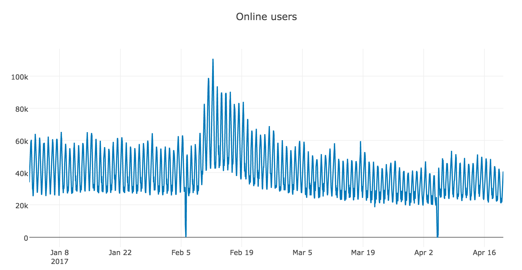
Rolling window estimations
Начнем моделирование с наивного предположения — «завтра будет, как вчера», но вместо модели вида  будем считать, что будущее значение переменной зависит от среднего
  её предыдущих значений, а значит, воспользуемся скользящей средней.

Реализуем эту же функцию в питоне и посмотрим на прогноз, построенный по последнему наблюдаемому дню (24 часа)
def moving_average(series, n):
    return np.average(series[-n:])

moving_average(dataset.Users, 24)
Out: 29858.333333333332К сожалению, такой прогноз долгосрочным сделать не удастся — для получения предсказания на шаг вперед предыдущее значение должно быть фактически наблюдаемой величиной. Зато у скользящей средней есть другое применение — сглаживание исходного ряда для выявления трендов. В пандасе есть готовая реализация — DataFrame.rolling(window).mean(). Чем больше зададим ширину интервала — тем более сглаженным окажется тренд. В случае, если данные сильно зашумлены, что особенно часто встречается, например, в финансовых показателях, такая процедура может помочь с определением общих паттернов.
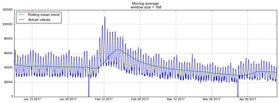
Для нашего ряда тренды и так вполне очевидны, но если сгладить по дням, становится лучше видна динамика онлайна по будням и выходным (выходные — время поиграть), а недельное сглаживание хорошо отражает общие изменения, связанные с резким ростом числа активных игроков в феврале и последующим снижением в марте.
Код для отрисовки графика
def plotMovingAverage(series, n):

    """
    series - dataframe with timeseries
    n - rolling window size

    """

    rolling_mean = series.rolling(window=n).mean()

    # При желании, можно строить и доверительные интервалы для сглаженных значений
    #rolling_std =  series.rolling(window=n).std()
    #upper_bond = rolling_mean+1.96*rolling_std
    #lower_bond = rolling_mean-1.96*rolling_std

    plt.figure(figsize=(15,5))
    plt.title("Moving averagen window size = {}".format(n))
    plt.plot(rolling_mean, "g", label="Rolling mean trend")

    #plt.plot(upper_bond, "r--", label="Upper Bond / Lower Bond")
    #plt.plot(lower_bond, "r--")
    plt.plot(dataset[n:], label="Actual values")
    plt.legend(loc="upper left")
    plt.grid(True)
plotMovingAverage(dataset, 24) # сглаживаем по дням
plotMovingAverage(dataset, 24*7) # сглаживаем по неделям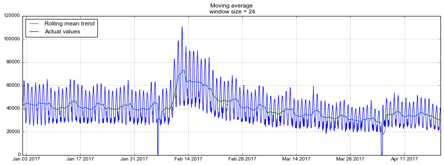
Модификацией простой скользящей средней является взвешенная средняя, внутри которой наблюдениям придаются различные веса, в сумме дающие единицу, при этом обычно последним наблюдениям присваивается больший вес.

def weighted_average(series, weights):
    result = 0.0
    weights.reverse()
    for n in range(len(weights)):
        result += series[-n-1] * weights[n]
    return result

weighted_average(dataset.Users, [0.6, 0.2, 0.1, 0.07, 0.03])
Out: 35967.550000000003Экспоненциальное сглаживание, модель Хольта-Винтерса
Простое экспоненциальное сглаживание
А теперь посмотрим, что произойдёт, если вместо взвешивания последних значений ряда мы начнем взвешивать все доступные наблюдения, при этом экспоненциально уменьшая веса по мере углубления в исторические данные. В этом нам поможет формула простого экспоненциального сглаживания:

Здесь модельное значение представляет собой средневзвешенную между текущим истинным и предыдущим модельным значениями. Вес  называется сглаживающим фактором. Он определяет, как быстро мы будем «забывать» последнее доступное истинное наблюдение. Чем меньше , тем больше влияния оказывают предыдущие модельные значения, и тем сильнее сглаживается ряд.
Экспоненциальность скрывается в рекурсивности функции — каждый раз мы умножаем  на предыдущее модельное значение, которое, в свою очередь, также содержало в себе , и так до самого начала.
def exponential_smoothing(series, alpha):
    result = [series[0]] # first value is same as series
    for n in range(1, len(series)):
        result.append(alpha * series[n] + (1 - alpha) * result[n-1])
    return result
Код для отрисовки графика
with plt.style.context('seaborn-white'):
    plt.figure(figsize=(20, 8))
    for alpha in [0.3, 0.05]:
        plt.plot(exponential_smoothing(dataset.Users, alpha), label="Alpha {}".format(alpha))
    plt.plot(dataset.Users.values, "c", label = "Actual")
    plt.legend(loc="best")
    plt.axis('tight')
    plt.title("Exponential Smoothing")
    plt.grid(True)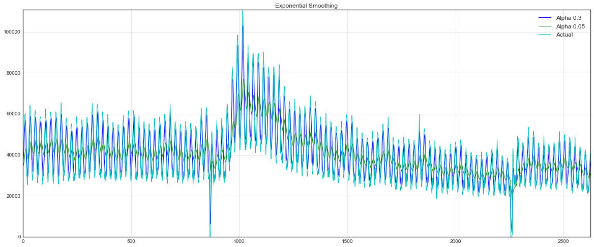
Двойное экспоненциальное сглаживание
До сих пор мы могли получить от наших методов в лучшем случае прогноз лишь на одну точку вперёд (и ещё красиво сгладить ряд), это здорово, но недостаточно, поэтому переходим к расширению экспоненциального сглаживания, которое позволит строить прогноз сразу на две точки вперед (и тоже красиво сглаживать ряд).
В этом нам поможет разбиение ряда на две составляющие — уровень (level, intercept)  и тренд
  (trend, slope). Уровень, или ожидаемое значение ряда, мы предсказывали при помощи предыдущих методов, а теперь такое же экспоненциальное сглаживание применим к тренду, наивно или не очень полагая, что будущее направление изменения ряда зависит от взвешенных предыдущих изменений.

В результате получаем набор функций. Первая описывает уровень — он, как и прежде, зависит от текущего значения ряда, а второе слагаемое теперь разбивается на предыдущее значение уровня и тренда. Вторая отвечает за тренд — он зависит от изменения уровня на текущем шаге, и от предыдущего значения тренда. Здесь в роли веса в экспоненциальном сглаживании выступает коэффициент  . Наконец, итоговое предсказание представляет собой сумму модельных значений уровня и тренда.
def double_exponential_smoothing(series, alpha, beta):
    result = [series[0]]
    for n in range(1, len(series)+1):
        if n == 1:
            level, trend = series[0], series[1] - series[0]
        if n >= len(series): # прогнозируем
            value = result[-1]
        else:
            value = series[n]
        last_level, level = level, alpha*value + (1-alpha)*(level+trend)
        trend = beta*(level-last_level) + (1-beta)*trend
        result.append(level+trend)
    return result
Код для отрисовки графика
with plt.style.context('seaborn-white'):
    plt.figure(figsize=(20, 8))
    for alpha in [0.9, 0.02]:
        for beta in [0.9, 0.02]:
            plt.plot(double_exponential_smoothing(dataset.Users, alpha, beta), label="Alpha {}, beta {}".format(alpha, beta))
    plt.plot(dataset.Users.values, label = "Actual")
    plt.legend(loc="best")
    plt.axis('tight')
    plt.title("Double Exponential Smoothing")
    plt.grid(True)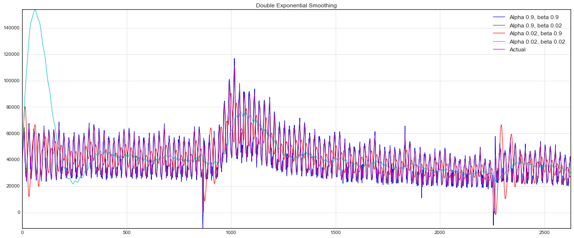
Теперь настраивать пришлось уже два параметра — и . Первый отвечает за сглаживание ряда вокруг тренда, второй — за сглаживание самого тренда. Чем выше значения, тем больший вес будет отдаваться последним наблюдениям и тем менее сглаженным окажется модельный ряд. Комбинации параметров могут выдавать достаточно причудливые результаты, особенно если задавать их руками. А о не ручном подборе параметров расскажу чуть ниже, сразу после тройного экспоненциального сглаживания.
Тройное экспоненциальное сглаживание a.k.a. Holt-Winters
Итак, успешно добрались до следующего варианта экспоненциального сглаживания, на сей раз тройного.
Идея этого метода заключается в добавлении еще одной, третьей, компоненты — сезонности. Соответственно, метод применим только в случае, если ряд этой сезонностью не обделён, что в нашем случае верно. Сезонная компонента в модели будет объяснять повторяющиеся колебания вокруг уровня и тренда, а характеризоваться она будет длиной сезона — периодом, после которого начинаются повторения колебаний. Для каждого наблюдения в сезоне формируется своя компонента, например, если длина сезона составляет 7 (например, недельная сезонность), то получим 7 сезонных компонент, по штуке на каждый из дней недели.
Получаем новую систему:

Уровень теперь зависит от текущего значения ряда за вычетом соответствующей сезонной компоненты, тренд остаётся без изменений, а сезонная компонента зависит от текущего значения ряда за вычетом уровня и от предыдущего значения компоненты. При этом компоненты сглаживаются через все доступные сезоны, например, если это компонента, отвечающая за понедельник, то и усредняться она будет только с другими понедельниками. Подробнее про работу усреднений и оценку начальных значений тренда и сезонных компонент можно почитать здесь. Теперь, имея сезонную компоненту, мы можем предсказывать уже не на один, и даже не на два, а на произвольные  шагов вперёд, что не может не радовать.
Ниже приведен код для построения модели тройного экспоненциального сглаживания, также известного по фамилиям её создателей — Чарльза Хольта и его студента Питера Винтерса.
Дополнительно в модель включен метод Брутлага для построения доверительных интервалов:

где  — длина сезона,
  — предсказанное отклонение, а остальные параметры берутся из тройного сглаживани. Подробнее о методе и о его применении к поиску аномалий во временных рядах можно прочесть здесь
Код для модели Хольта-Винтерса
class HoltWinters:

    """
    Модель Хольта-Винтерса с методом Брутлага для детектирования аномалий
    https://fedcsis.org/proceedings/2012/pliks/118.pdf

    # series - исходный временной ряд
    # slen - длина сезона
    # alpha, beta, gamma - коэффициенты модели Хольта-Винтерса
    # n_preds - горизонт предсказаний
    # scaling_factor - задаёт ширину доверительного интервала по Брутлагу (обычно принимает значения от 2 до 3)

    """

    def __init__(self, series, slen, alpha, beta, gamma, n_preds, scaling_factor=1.96):
        self.series = series
        self.slen = slen
        self.alpha = alpha
        self.beta = beta
        self.gamma = gamma
        self.n_preds = n_preds
        self.scaling_factor = scaling_factor

    def initial_trend(self):
        sum = 0.0
        for i in range(self.slen):
            sum += float(self.series[i+self.slen] - self.series[i]) / self.slen
        return sum / self.slen

    def initial_seasonal_components(self):
        seasonals = {}
        season_averages = []
        n_seasons = int(len(self.series)/self.slen)
        # вычисляем сезонные средние
        for j in range(n_seasons):
            season_averages.append(sum(self.series[self.slen*j:self.slen*j+self.slen])/float(self.slen))
        # вычисляем начальные значения
        for i in range(self.slen):
            sum_of_vals_over_avg = 0.0
            for j in range(n_seasons):
                sum_of_vals_over_avg += self.series[self.slen*j+i]-season_averages[j]
            seasonals[i] = sum_of_vals_over_avg/n_seasons
        return seasonals

    def triple_exponential_smoothing(self):
        self.result = []
        self.Smooth = []
        self.Season = []
        self.Trend = []
        self.PredictedDeviation = []
        self.UpperBond = []
        self.LowerBond = []

        seasonals = self.initial_seasonal_components()

        for i in range(len(self.series)+self.n_preds):
            if i == 0: # инициализируем значения компонент
                smooth = self.series[0]
                trend = self.initial_trend()
                self.result.append(self.series[0])
                self.Smooth.append(smooth)
                self.Trend.append(trend)
                self.Season.append(seasonals[i%self.slen])

                self.PredictedDeviation.append(0)

                self.UpperBond.append(self.result[0] +
                                      self.scaling_factor *
                                      self.PredictedDeviation[0])

                self.LowerBond.append(self.result[0] -
                                      self.scaling_factor *
                                      self.PredictedDeviation[0])

                continue
            if i >= len(self.series): # прогнозируем
                m = i - len(self.series) + 1
                self.result.append((smooth + m*trend) + seasonals[i%self.slen])

                # во время прогноза с каждым шагом увеличиваем неопределенность
                self.PredictedDeviation.append(self.PredictedDeviation[-1]*1.01)

            else:
                val = self.series[i]
                last_smooth, smooth = smooth, self.alpha*(val-seasonals[i%self.slen]) + (1-self.alpha)*(smooth+trend)
                trend = self.beta * (smooth-last_smooth) + (1-self.beta)*trend
                seasonals[i%self.slen] = self.gamma*(val-smooth) + (1-self.gamma)*seasonals[i%self.slen]
                self.result.append(smooth+trend+seasonals[i%self.slen])

                # Отклонение рассчитывается в соответствии с алгоритмом Брутлага
                self.PredictedDeviation.append(self.gamma * np.abs(self.series[i] - self.result[i])
                                               + (1-self.gamma)*self.PredictedDeviation[-1])

            self.UpperBond.append(self.result[-1] +
                                  self.scaling_factor *
                                  self.PredictedDeviation[-1])

            self.LowerBond.append(self.result[-1] -
                                  self.scaling_factor *
                                  self.PredictedDeviation[-1])

            self.Smooth.append(smooth)
            self.Trend.append(trend)
            self.Season.append(seasonals[i % self.slen])
Кросс-валидация на временных рядах, подбор параметров
Перед тем, как построить модель, поговорим, наконец, о не ручной оценке параметров для моделей.
Ничего необычного здесь нет, по-прежнему сначала необходимо выбрать подходящуюю для данной задачи функцию потерь: RMSE, MAE, MAPE и др., которая будет следить за качеством подгонки модели под исходные данные. Затем будем оценивать на кросс-валидации значение функции потерь при данных параметрах модели, искать градиент, менять в соответствии с ним параметры и бодро опускаться в сторону глобального минимума ошибки.
Небольшая загвоздка возникает только в кросс-валидации. Проблема состоит в том, что временной ряд имеет, как ни парадоксально, временную структуру, и случайно перемешивать в фолдах значения всего ряда без сохранения этой структуры нельзя, иначе в процессе потеряются все взаимосвязи наблюдений друг с другом. Поэтому придется использовать чуть более хитрый способ для оптимизации параметров, официального названия которому я так и не нашел, но на сайте CrossValidated, где можно найти ответы на всё, кроме главного вопроса Жизни, Вселенной и Всего Остального, предлагают название «cross-validation on a rolling basis», что не дословно можно перевести как кросс-валидация на скользящем окне.
Суть достаточно проста — начинаем обучать модель на небольшом отрезке временного ряда, от начала до некоторого  , делаем прогноз на
  шагов вперед и считаем ошибку. Далее расширяем обучающую выборку до значения и прогнозируем с до
  , так продолжаем двигать тестовый отрезок ряда до тех пор, пока не упрёмся в последнее доступное наблюдение. В итоге получим столько фолдов, сколько уместится в промежуток между изначальным обучающим отрезком и всей длиной ряда.
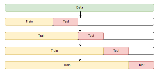
Код для кросс-валидации на временном ряду
from sklearn.model_selection import TimeSeriesSplit

def timeseriesCVscore(x):
    # вектор ошибок
    errors = []

    values = data.values
    alpha, beta, gamma = x

    # задаём число фолдов для кросс-валидации
    tscv = TimeSeriesSplit(n_splits=3)

    # идем по фолдам, на каждом обучаем модель, строим прогноз на отложенной выборке и считаем ошибку
    for train, test in tscv.split(values):

        model = HoltWinters(series=values[train], slen = 24*7, alpha=alpha, beta=beta, gamma=gamma, n_preds=len(test))
        model.triple_exponential_smoothing()

        predictions = model.result[-len(test):]
        actual = values[test]
        error = mean_squared_error(predictions, actual)
        errors.append(error)

    # Возвращаем средний квадрат ошибки по вектору ошибок
    return np.mean(np.array(errors))
Значение длины сезона 24*7 возникло не случайно — в исходном ряде отчетливо видна дневная сезонность, (отсюда 24), и недельная — по будням ниже, на выходных — выше, (отсюда 7), суммарно сезонных компонент получится 24*7.
В модели Хольта-Винтерса, как и в остальных моделях экспоненциального сглаживания, есть ограничение на величину сглаживающих параметров — каждый из них может принимать значения от 0 до 1, поэтому для минимизации функции потерь нужно выбирать алгоритм, поддерживающий ограничения на параметры, в данном случае — Truncated Newton conjugate gradient.
%%time
data = dataset.Users[:-500] # отложим часть данных для тестирования

# инициализируем значения параметров
x = [0, 0, 0]

# Минимизируем функцию потерь с ограничениями на параметры
opt = minimize(timeseriesCVscore, x0=x, method="TNC", bounds = ((0, 1), (0, 1), (0, 1)))

# Из оптимизатора берем оптимальное значение параметров
alpha_final, beta_final, gamma_final = opt.x
print(alpha_final, beta_final, gamma_final)
Out: (0.0066342670643441681, 0.0, 0.046765204289672901)Передадим полученные оптимальные значения коэффициентов , и  и построим прогноз на 5 дней вперёд (128 часов)
# Передаем оптимальные значения модели,
data = dataset.Users
model = HoltWinters(data[:-128], slen = 24*7, alpha = alpha_final, beta = beta_final, gamma = gamma_final, n_preds = 128, scaling_factor = 2.56)
model.triple_exponential_smoothing()
Код для отрисовки графика
def plotHoltWinters():
    Anomalies = np.array([np.NaN]*len(data))
    Anomalies[data.values<model.LowerBond] = data.values[data.values<model.LowerBond]
    plt.figure(figsize=(25, 10))
    plt.plot(model.result, label = "Model")
    plt.plot(model.UpperBond, "r--", alpha=0.5, label = "Up/Low confidence")
    plt.plot(model.LowerBond, "r--", alpha=0.5)
    plt.fill_between(x=range(0,len(model.result)), y1=model.UpperBond, y2=model.LowerBond, alpha=0.5, color = "grey")
    plt.plot(data.values, label = "Actual")
    plt.plot(Anomalies, "o", markersize=10, label = "Anomalies")
    plt.axvspan(len(data)-128, len(data), alpha=0.5, color='lightgrey')
    plt.grid(True)
    plt.axis('tight')
    plt.legend(loc="best", fontsize=13);

plotHoltWinters()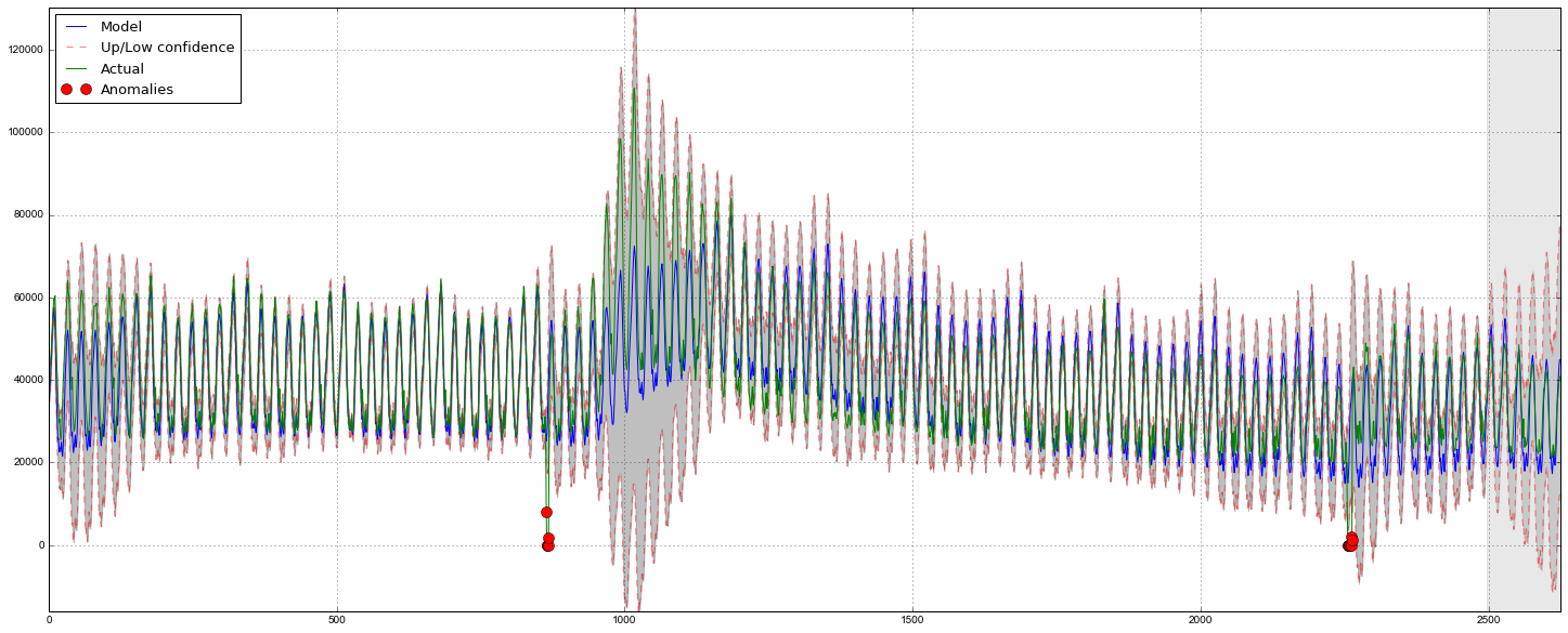
Судя по графику, модель неплохо описала исходный временной ряд, уловив недельную и дневную сезонность, и даже смогла поймать аномальные снижения, вышедшие за пределы доверительных интервалов. Если посмотреть на смоделированное отклонение, хорошо видно, что модель достаточно резко регирует на значительные изменения в структуре ряда, но при этом быстро возвращает дисперсию к обычным значениям, «забывая» прошлое. Такая особенность позволяет неплохо и без значительных затрат на подготовку-обучение модели настроить систему по детектированию аномалий даже в достаточно шумных рядах.
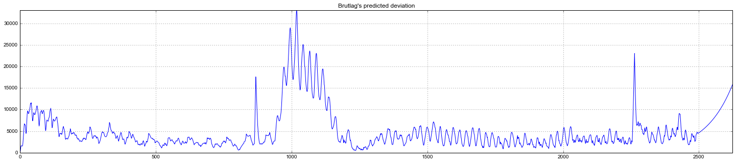
Эконометрический подход
Стационарность, единичные корни
Перед тем, как перейти к моделированию, стоит сказать о таком важном свойстве временного ряда, как стационарность.
Под стационарностью понимают свойство процесса не менять своих статистических характеристик с течением времени, а именно постоянство матожидания, постоянство дисперсии (она же гомоскедастичность) и независимость ковариационной функции от времени (должна зависеть только от расстояния между наблюдениями). Наглядно можно посмотреть на эти свойства на картинках, взятых из поста Sean Abu:
- Временной ряд справа не является стационарным, так как его матожидание со временем растёт
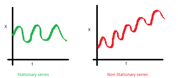
- Здесь не повезло с дисперсией — разброс значений ряда существенно варьируется в зависимости от периода
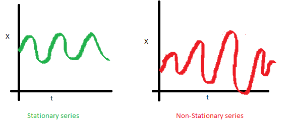
- Наконец, на последнем графике видно, что значения ряда внезапно становятся ближе друг ко другу, образуя некоторый кластер, а в результате получаем непостоянство ковариаций
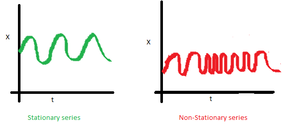
Почему стационарность так важна? По стационарному ряду просто строить прогноз, так как мы полагаем, что его будущие статистические характеристики не будут отличаться от наблюдаемых текущих. Большинство моделей временных рядов так или иначе моделируют и предсказывают эти характеристики (например, матожидание или дисперсию), поэтому в случае нестационарности исходного ряда предсказания окажутся неверными. К сожалению, большинство временных рядов, с которыми приходится сталкиваться за пределыми учебных материалов, стационарными не являются, но с этим можно (и нужно) бороться.
Чтобы бороться с нестационарностью, нужно узнать её в лицо, потому посмотрим, как её детектировать. Для этого обратимся к белому шуму и случайному блужданию, чтобы выяснить как попасть из одного в другое бесплатно и без смс.
График белого шума:
white_noise = np.random.normal(size=1000)
with plt.style.context('bmh'):
    plt.figure(figsize=(15, 5))
    plt.plot(white_noise)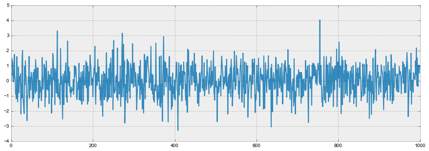
Итак, процесс, порожденный стандартным нормальным распределением, стационарен, колеблется вокруг нуля с отклонением в 1. Теперь на основании него сгенерируем новый процесс, в котором каждое последующее значение будет зависеть от предыдущего: 
Код для отрисовки графиков
def plotProcess(n_samples=1000, rho=0):
    x = w = np.random.normal(size=n_samples)
    for t in range(n_samples):
        x[t] = rho * x[t-1] + w[t]

    with plt.style.context('bmh'):
        plt.figure(figsize=(10, 3))
        plt.plot(x)
        plt.title("Rho {}n Dickey-Fuller p-value: {}".format(rho, round(sm.tsa.stattools.adfuller(x)[1], 3)))

for rho in [0, 0.6, 0.9, 1]:
    plotProcess(rho=rho)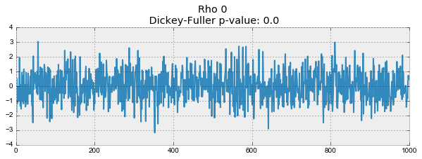
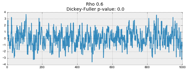
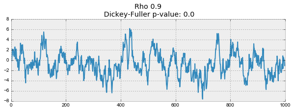
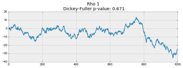
На первом графике получился точно такой же стационарный белый шум, который строился раньше. На втором значение  увеличилось до 0.6, в результате чего на графике стали появляться более широкие циклы, но в целом стационарным он быть пока не перестал. Третий график всё сильнее отклоняется от нулевого среднего значения, но всё ещё колеблется вокруг него. Наконец, значение равное единице дало процесс случайного блуждания — ряд не стационарен.
Происходит это из-за того, что при достижении критической единицы, ряд перестаёт возвращаться к своему среднему значению. Если вычесть из левой и правой части  , то получим
  , где выражение слева — первые разности. Если
  , то первые разности дадут стационарный белый шум
  . Этот факт лёг в основу теста Дики-Фуллера на стационарность ряда (наличие единичного корня). Если из нестационарного ряда первыми разностями удаётся получить стационарный, то он называется интегрированным первого порядка. Нулевая гипотеза теста — ряд не стационарен, отвергалась на первых трех графиках, и принялась на последнем. Стоит сказать, что не всегда для получения стационарного ряда хватает первых разностей, так как процесс может быть интегрированным с более высоким порядком (иметь несколько единичных корней), для проверки таких случаев используют расширенный тест Дики-Фуллера, проверяющий сразу несколько лагов.
Бороться с нестационарностью можно множеством способов — разностями различного порядка, выделением тренда и сезонности, сглаживаниями и преобразованиями, например, Бокса-Кокса или логарифмированием.
Избавляемся от нестационарности и строим SARIMA
Попробуем теперь построить ARIMA модель для онлайна игроков, пройдя все круги ада стадии приведения ряда к стационарному виду. Про саму модель уже не раз писали на хабре — Построение модели SARIMA с помощью Python+R, Анализ временных рядов с помощью python, поэтому подробно останавливаться на ней не буду.
Код для отрисовки графиков
def tsplot(y, lags=None, figsize=(12, 7), style='bmh'):
    if not isinstance(y, pd.Series):
        y = pd.Series(y)
    with plt.style.context(style):
        fig = plt.figure(figsize=figsize)
        layout = (2, 2)
        ts_ax = plt.subplot2grid(layout, (0, 0), colspan=2)
        acf_ax = plt.subplot2grid(layout, (1, 0))
        pacf_ax = plt.subplot2grid(layout, (1, 1))

        y.plot(ax=ts_ax)
        ts_ax.set_title('Time Series Analysis Plots')
        smt.graphics.plot_acf(y, lags=lags, ax=acf_ax, alpha=0.5)
        smt.graphics.plot_pacf(y, lags=lags, ax=pacf_ax, alpha=0.5)

        print("Критерий Дики-Фуллера: p=%f" % sm.tsa.stattools.adfuller(y)[1])

        plt.tight_layout()
    return

tsplot(dataset.Users, lags=30)
Out: Критерий Дики-Фуллера: p=0.190189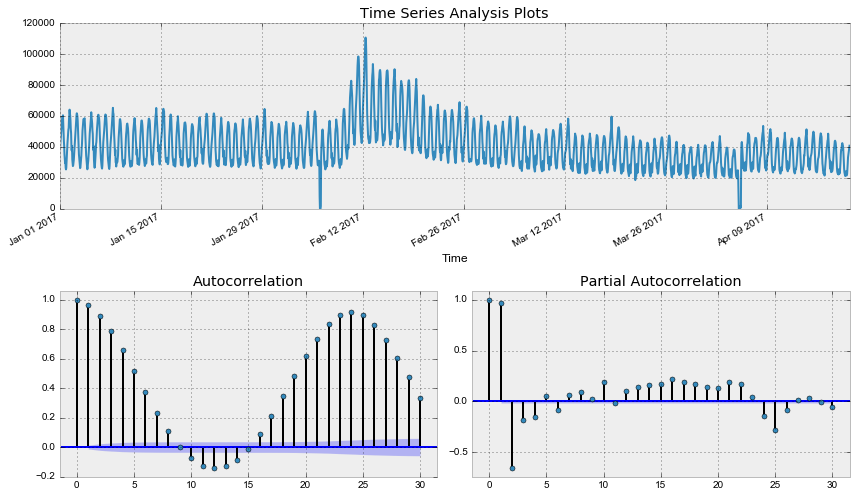
Как и следовало ожидать, исходный ряд стационарным не является, критерий Дики-Фуллера не отверг нулевую гипотезу о наличии единичного корня. Попробуем стабилизировать дисперсию преоразованием Бокса-Кокса.
def invboxcox(y,lmbda):
    # обрабтное преобразование Бокса-Кокса
    if lmbda == 0:
        return(np.exp(y))
    else:
        return(np.exp(np.log(lmbda*y+1)/lmbda))

data = dataset.copy()
data['Users_box'], lmbda = scs.boxcox(data.Users+1) # прибавляем единицу, так как в исходном ряде есть нули
tsplot(data.Users_box, lags=30)
print("Оптимальный параметр преобразования Бокса-Кокса: %f" % lmbda)
Out: Критерий Дики-Фуллера: p=0.079760
Оптимальный параметр преобразования Бокса-Кокса: 0.587270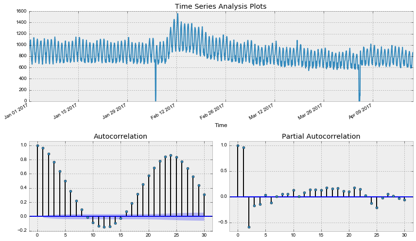
Уже лучше, однако критерий Дики-Фуллера по-прежнему не отвергает гипотезу о нестационарности ряда. А автокорреляционная функция явно намекает на сезонность в получившемся ряде. Возьмём сезонные разности:
data['Users_box_season'] = data.Users_box - data.Users_box.shift(24*7)
tsplot(data.Users_box_season[24*7:], lags=30)
Out: Критерий Дики-Фуллера: p=0.002571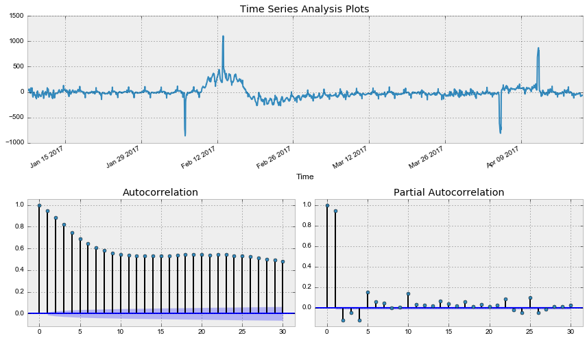
Критерий Дики-Фуллера теперь отвергает нулевую гипотезу о нестационарности, но автокорреляционная функция всё ещё выглядит нехорошо из-за большого числа значимых лагов. Так как на графике частной автокорреляционной функции значим лишь один лаг, стоит взять еще первые разности, чтобы привести наконец ряд к стационарному виду.
data['Users_box_season_diff'] = data.Users_box_season - data.Users_box_season.shift(1)
tsplot(data.Users_box_season_diff[24*7+1:], lags=30)
Out: Критерий Дики-Фуллера: p=0.000000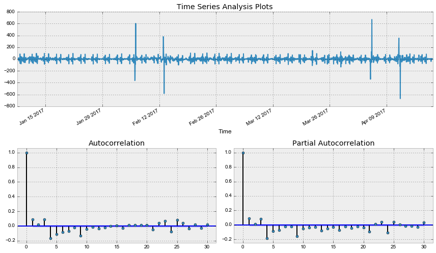
Наконец, получили стационарный ряд, по автокорреляционной и частной автокорреляционной функции прикинем параметры для SARIMA модели, на забыв, что предварительно уже сделали первые и сезонные разности.
Начальные приближения Q = 1, P = 4, q = 3, p = 4
ps = range(0, 5)
d=1
qs = range(0, 4)
Ps = range(0, 5)
D=1
Qs = range(0, 1)

from itertools import product

parameters = product(ps, qs, Ps, Qs)
parameters_list = list(parameters)
len(parameters_list)
Out: 100Код для подбора параметров перебором
%%time
results = []
best_aic = float("inf")

for param in tqdm(parameters_list):
    #try except нужен, потому что на некоторых наборах параметров модель не обучается
    try:
        model=sm.tsa.statespace.SARIMAX(data.Users_box, order=(param[0], d, param[1]),
                                        seasonal_order=(param[2], D, param[3], 24*7)).fit(disp=-1)
    #выводим параметры, на которых модель не обучается и переходим к следующему набору
    except ValueError:
        print('wrong parameters:', param)
        continue
    aic = model.aic
    #сохраняем лучшую модель, aic, параметры
    if aic < best_aic:
        best_model = model
        best_aic = aic
        best_param = param
    results.append([param, model.aic])

warnings.filterwarnings('default')

result_table = pd.DataFrame(results)
result_table.columns = ['parameters', 'aic']
print(result_table.sort_values(by = 'aic', ascending=True).head())
Лучшие параметры загоняем в модель:
%%time
best_model = sm.tsa.statespace.SARIMAX(data.Users_box, order=(4, d, 3),
                                        seasonal_order=(4, D, 1, 24)).fit(disp=-1)
print(best_model.summary())
Statespace Model Results
==========================================================================================
Dep. Variable: Users_box No. Observations: 2625
Model: SARIMAX(4, 1, 3)x(4, 1, 1, 24) Log Likelihood -12547.157
Date: Sun, 23 Apr 2017 AIC 25120.315
Time: 02:06:39 BIC 25196.662
Sample: 0 HQIC 25147.964
- 2625
Covariance Type: opg
==============================================================================
coef std err z P>|z| [0.025 0.975]
------------------------------------------------------------------------------
ar.L1 0.6794 0.108 6.310 0.000 0.468 0.890
ar.L2 -0.0810 0.181 -0.448 0.654 -0.435 0.273
ar.L3 0.3255 0.137 2.371 0.018 0.056 0.595
ar.L4 -0.2154 0.028 -7.693 0.000 -0.270 -0.161
ma.L1 -0.5086 0.106 -4.784 0.000 -0.717 -0.300
ma.L2 -0.0673 0.170 -0.395 0.693 -0.401 0.267
ma.L3 -0.3490 0.117 -2.976 0.003 -0.579 -0.119
ar.S.L24 0.1023 0.012 8.377 0.000 0.078 0.126
ar.S.L48 -0.0686 0.021 -3.219 0.001 -0.110 -0.027
ar.S.L72 0.1971 0.009 21.573 0.000 0.179 0.215
ar.S.L96 -0.1217 0.013 -9.279 0.000 -0.147 -0.096
ma.S.L24 -0.9983 0.045 -22.085 0.000 -1.087 -0.910
sigma2 873.4159 36.206 24.124 0.000 802.454 944.378
===================================================================================
Ljung-Box (Q): 130.47 Jarque-Bera (JB): 1194707.99
Prob(Q): 0.00 Prob(JB): 0.00
Heteroskedasticity (H): 1.40 Skew: 2.65
Prob(H) (two-sided): 0.00 Kurtosis: 107.88
===================================================================================
Warnings:
[1] Covariance matrix calculated using the outer product of gradients (complex-step).Проверим остатки модели:
tsplot(best_model.resid[24:], lags=30)Out: Критерий Дики-Фуллера: p=0.000000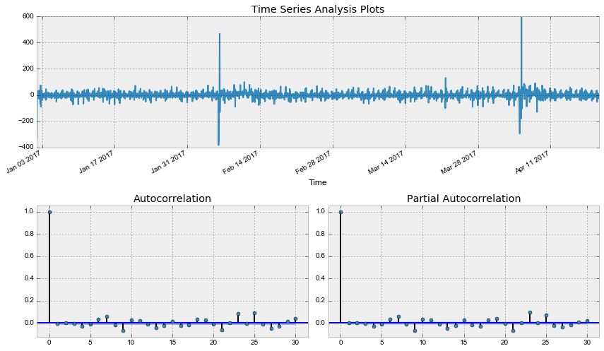
Что ж, остатки стационарны, явных автокорреляций нет, построим прогноз по получившейся модели
Код для построения прогноза и отрисовки графика
data["arima_model"] = invboxcox(best_model.fittedvalues, lmbda)
forecast = invboxcox(best_model.predict(start = data.shape[0], end = data.shape[0]+100), lmbda)
forecast = data.arima_model.append(forecast).values[-500:]
actual = data.Users.values[-400:]
plt.figure(figsize=(15, 7))
plt.plot(forecast, color='r', label="model")
plt.title("SARIMA modeln Mean absolute error {} users".format(round(mean_absolute_error(data.dropna().Users, data.dropna().arima_model))))
plt.plot(actual, label="actual")
plt.legend()
plt.axvspan(len(actual), len(forecast), alpha=0.5, color='lightgrey')
plt.grid(True)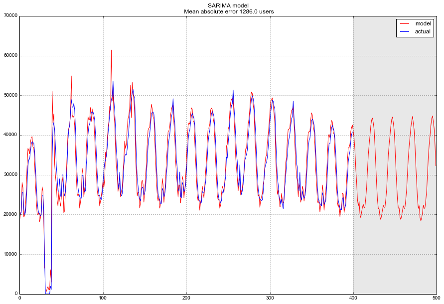
В финале получаем достаточно адекватный прогноз, в среднем модель ошибалась на 1.3 K пользователей, что очень и очень неплохо, однако суммарные затраты на подготовку данных, приведение к стационарности, определение и перебор параметров могут такой точности и не стоить.
Линейные и не очень модели на временных рядах
Снова небольшое лирическое отступление. Часто на работе приходится строить модели, руководствуясь одним основополагающим принципом – быстро, качественно, недорого. Поэтому часть моделей могут банально не подойти для «продакшн-решений», так как либо требуют слишком больших затрат по подготовке данных (например, SARIMA), либо сложно настраиваются (хороший пример – SARIMA), либо требуют частого переобучения на новых данных (опять SARIMA), поэтому зачастую гораздо проще бывает выделить несколько признаков из имеющегося временного ряда и построить по ним обычную линейную регрессию или навесить решаюший лес. Дешево и сердито.
Возможно, этот подход не является значительно подкрепленным теорией, нарушает различные предпосылки, например, условия Гаусса-Маркова, особенно пункт про некоррелированность ошибок, однако на практике нередко выручает и достаточно активно используется в соревнованиях по машинному обучению.
Помимо стандартных признаков вроде лагов целевой переменной, много информации содержат в себе дата и время. Про извлечение признаков из них уже здорово описано в одной из предыдущих статей курса.
Добавлю только про еще один вариант кодирования категориальных признаков – кодирование средним. Если не хочется раздувать датасет множеством дамми-переменных, которые могут привести к потере информации о расстоянии, а в вещественном виде возникают противоречивые результаты а-ля «0 часов < 23 часа», то можно закодировать переменную чуть более интерпретируемыми значениями. Естественный вариант – закодировать средним значением целевой переменной. В нашем случае каждый день недели или час дня можно закодировать сооветствующим средним числом игроков, находившихся в этот день недели или час онлайн. При этом важно следить за тем, чтобы расчет среднего значения производился только в рамках тестового датасета (или в рамках текущего наблюдаемого фолда при кросс-валидации), иначе можно ненароком привнести в модель информацию о будущем.
def code_mean(data, cat_feature, real_feature):
    """
    Возвращает словарь, где ключами являются уникальные категории признака cat_feature,
    а значениями - средние по real_feature
    """
    return dict(data.groupby(cat_feature)[real_feature].mean())
Создадим новый датафрейм и добавим в него час, день недели и выходной в качестве категориальных переменных. Для этого переводим имеющийся в датафрейме индекс в формат datetime, и извлекаем из него hour и weekday.
data = pd.DataFrame(dataset)
data.columns = ["y"]

data.index = data.index.to_datetime()
data["hour"] = data.index.hour
data["weekday"] = data.index.weekday
data['is_weekend'] = data.weekday.isin([5,6])*1
data.head()Out:Посмотрим на средние по дням недели
code_mean(data, 'weekday', "y")Out:
{0: 38730.143229166664,
1: 38632.828125,
2: 38128.518229166664,
3: 39519.035135135135,
4: 41505.152777777781,
5: 43717.708333333336,
6: 43392.143603133161}Помимо перечисленных преобразований для увеличения числа признаков используют и множество других метрик, например, максимальное/минимальное значение, наблюдавшееся в скользящем по ряду окне, медианы, число пиков, взвешенные дисперсии и многое другое. Автоматически этим занимается уже упоминавшаяся в курсе библиотека библиотека tsfresh.
Для удобства все преобразования можно записать в одну функцию, которая сразу же будет возвращать разбитые на трейн и тест датасеты и целевые переменные.
Функция для создания переменных
def prepareData(data, lag_start=5, lag_end=20, test_size=0.15):

    data = pd.DataFrame(data.copy())
    data.columns = ["y"]

    # считаем индекс в датафрейме, после которого начинается тестовыый отрезок
    test_index = int(len(data)*(1-test_size))

    # добавляем лаги исходного ряда в качестве признаков
    for i in range(lag_start, lag_end):
        data["lag_{}".format(i)] = data.y.shift(i)

    data.index = data.index.to_datetime()
    data["hour"] = data.index.hour
    data["weekday"] = data.index.weekday
    data['is_weekend'] = data.weekday.isin([5,6])*1

    # считаем средние только по тренировочной части, чтобы избежать лика
    data['weekday_average'] = map(code_mean(data[:test_index], 'weekday', "y").get, data.weekday)
    data["hour_average"] = map(code_mean(data[:test_index], 'hour', "y").get, data.hour)

    # выкидываем закодированные средними признаки
    data.drop(["hour", "weekday"], axis=1, inplace=True)

    data = data.dropna()
    data = data.reset_index(drop=True)

    # разбиваем весь датасет на тренировочную и тестовую выборку
    X_train = data.loc[:test_index].drop(["y"], axis=1)
    y_train = data.loc[:test_index]["y"]
    X_test = data.loc[test_index:].drop(["y"], axis=1)
    y_test = data.loc[test_index:]["y"]

    return X_train, X_test, y_train, y_test
Линейная регрессия vs XGBoost
Обучим на получившихся данных простую линейную регрессию. При этом лаги будем брать начиная с двенадцатого, таким образом модель будет способна строить предсказания на 12 часов вперёд, имея фактические наблюдения за предыдущие пол дня.
Построение линейной регрессии
from sklearn.linear_model import LinearRegression

X_train, X_test, y_train, y_test = prepareData(dataset.Users, test_size=0.3, lag_start=12, lag_end=48)
lr = LinearRegression()
lr.fit(X_train, y_train)
prediction = lr.predict(X_test)
plt.figure(figsize=(15, 7))
plt.plot(prediction, "r", label="prediction")
plt.plot(y_test.values, label="actual")
plt.legend(loc="best")
plt.title("Linear regressionn Mean absolute error {} users".format(round(mean_absolute_error(prediction, y_test))))
plt.grid(True);
Получилось достаточно неплохо, даже отбора признаков модель ошибается, в среднем, на 3K пользователей в час, и это учитывая огромный выброс в середине тестового ряда.
Также можно провести оценку модели на кросс-валидации, тому же принципу, что был использован ранее. Для этого воспользуемся функцией (с небольшими модификациями), предложенной в посте Pythonic Cross Validation on Time Series
Код для кросс-валидации
def performTimeSeriesCV(X_train, y_train, number_folds, model, metrics):
    print('Size train set: {}'.format(X_train.shape))

    k = int(np.floor(float(X_train.shape[0]) / number_folds))
    print('Size of each fold: {}'.format(k))

    errors = np.zeros(number_folds-1)

    # loop from the first 2 folds to the total number of folds
    for i in range(2, number_folds + 1):
        print('')
        split = float(i-1)/i
        print('Splitting the first ' + str(i) + ' chunks at ' + str(i-1) + '/' + str(i) )

        X = X_train[:(k*i)]
        y = y_train[:(k*i)]
        print('Size of train + test: {}'.format(X.shape)) # the size of the dataframe is going to be k*i

        index = int(np.floor(X.shape[0] * split))

        # folds used to train the model
        X_trainFolds = X[:index]
        y_trainFolds = y[:index]

        # fold used to test the model
        X_testFold = X[(index + 1):]
        y_testFold = y[(index + 1):]

        model.fit(X_trainFolds, y_trainFolds)
        errors[i-2] = metrics(model.predict(X_testFold), y_testFold)

    # the function returns the mean of the errors on the n-1 folds
    return errors.mean()
%%time
performTimeSeriesCV(X_train, y_train, 5, lr, mean_absolute_error)Size train set: (1838, 39)
Size of each fold: 367
Splitting the first 2 chunks at 1/2
Size of train + test: (734, 39)
Splitting the first 3 chunks at 2/3
Size of train + test: (1101, 39)
Splitting the first 4 chunks at 3/4
Size of train + test: (1468, 39)
Splitting the first 5 chunks at 4/5
Size of train + test: (1835, 39)
CPU times: user 59.5 ms, sys: 7.02 ms, total: 66.5 ms
Wall time: 18.9 ms
Out: 4613.17893150896
На 5 фолдах получили среднюю абсолютную ошибку в 4.6 K пользователей, достаточно близко к оценке качества, полученной на тестовом датасете.
Почему бы теперь не попробовать XGBoost…

Код для построения прогноза с XGBoost
import xgboost as xgb

def XGB_forecast(data, lag_start=5, lag_end=20, test_size=0.15, scale=1.96):

    # исходные данные
    X_train, X_test, y_train, y_test = prepareData(dataset.Users, lag_start, lag_end, test_size)
    dtrain = xgb.DMatrix(X_train, label=y_train)
    dtest = xgb.DMatrix(X_test)

    # задаём параметры
    params = {
        'objective': 'reg:linear',
        'booster':'gblinear'
    }
    trees = 1000

    # прогоняем на кросс-валидации с метрикой rmse
    cv = xgb.cv(params, dtrain, metrics = ('rmse'), verbose_eval=False, nfold=10, show_stdv=False, num_boost_round=trees)

    # обучаем xgboost с оптимальным числом деревьев, подобранным на кросс-валидации
    bst = xgb.train(params, dtrain, num_boost_round=cv['test-rmse-mean'].argmin())

    # можно построить кривые валидации
    #cv.plot(y=['test-mae-mean', 'train-mae-mean'])

    # запоминаем ошибку на кросс-валидации
    deviation = cv.loc[cv['test-rmse-mean'].argmin()]["test-rmse-mean"]

    # посмотрим, как модель вела себя на тренировочном отрезке ряда
    prediction_train = bst.predict(dtrain)
    plt.figure(figsize=(15, 5))
    plt.plot(prediction_train)
    plt.plot(y_train)
    plt.axis('tight')
    plt.grid(True)

    # и на тестовом
    prediction_test = bst.predict(dtest)
    lower = prediction_test-scale*deviation
    upper = prediction_test+scale*deviation

    Anomalies = np.array([np.NaN]*len(y_test))
    Anomalies[y_test<lower] = y_test[y_test<lower]

    plt.figure(figsize=(15, 5))
    plt.plot(prediction_test, label="prediction")
    plt.plot(lower, "r--", label="upper bond / lower bond")
    plt.plot(upper, "r--")
    plt.plot(list(y_test), label="y_test")
    plt.plot(Anomalies, "ro", markersize=10)
    plt.legend(loc="best")
    plt.axis('tight')
    plt.title("XGBoost Mean absolute error {} users".format(round(mean_absolute_error(prediction_test, y_test))))
    plt.grid(True)
    plt.legend()
XGB_forecast(dataset, test_size=0.2, lag_start=5, lag_end=30)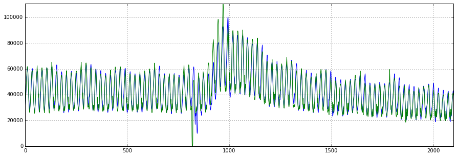

Те же 3 K пользователей в средней абсолютной ошибке, и неплохо пойманные аномалии на тестовом датасете. Конечно, чтобы уменьшить ошибку, еще можно повозиться с параметрами, настроить при необходимости регуляризацию, отобрать признаки, понять, на сколько лагов нужно уходить вглубь истории и т.д.
Заключение
Мы познакомились с разными методами и подходами к анализу и прогнозированию временных рядов. К сожалению, или к счастью, серебряной пули для решения такого рода задач пока не появилось. Методы, разработанные в 60-е годы прошлого века, (а некоторые и в начале 19-го), по-прежнему пользуются популярностью наравне с неразобранными в рамках данной статьи LSTM или RNN. Отчасти это связано с тем, что задача прогнозирования, как и любая другая задача, возникающая в процессе работы с данными — во многом творческая и уж точно исследовательская. Несмотря на обилие формальных метрик качества и способов оценки параметров, для каждого временного ряда часто приходится подбирать и пробовать что-то своё. Не последнюю роль играет и баланс между качеством и трудозатратами. Не раз уже упоминавшаяся здесь SARIMA-модель хотя и демонстрирует выдающиеся результаты при должной настройке, может потребовать не одного часа танцев с бубном манипуляций с рядом, в то время как простенькую линейную регрессию можно соорудить за 10 минут, получив при этом более-менее сравнимые результаты.
Домашнее задание №9
В демо-версии домашнего задания вы будете предсказывать просмотры wiki-страницы «Machine Learning». Веб-форма для ответов, там же найдете и решение.
Актуальные и обновляемые версии демо-заданий – на английском на сайте курса, вот первое задание. Также по подписке на Patreon («Bonus Assignments» tier) доступны расширенные домашние задания по каждой теме (только на англ.).
Полезные ресурсы
- Open Machine Learning Course. Topic 9. Part 1. Time series analysis in Python
- Видеозапись лекции по мотивам этой статьи
- Open Machine Learning Course. Topic 9. Part 2. Predicting the future with Facebook Prophet
- Онлайн-учебник курса по продвинутому статистическому прогнозированию университета Duke — разобраны всевозможные сглаживания, линейные модели и ARIMA модели
- Статья Comparison of ARIMA and Random Forest time series models for prediction of avian influenza H5N1 outbreaks — одна из немногих, где активно защищается позиция случайного леса в задачах по прогнозированию временных рядов
- Статья Time Series Analysis (TSA) in Python — Linear Models to GARCH семействе моделей ARIMA и их применении для моделирования финансовых показателей (Brian Christopher)
Материал статьи доступен в GitHub-репозитории курса
в виде тетрадок Jupyter.
https://gist.github.com/yogabonito/5461b26bed335cad6907aa4e613acb99
In this git link they implement a model using VECM in python
Some important parts of code are here
%matplotlib inline
import pandas
from statsmodels.tsa.vecm.vecm import VECM, select_order
import data as dta
iidata = dta.load_pandas();
mdata = iidata.data
dates = mdata[['year', 'quarter']].astype(int).astype(str)
quarterly = dates["year"] + "Q" + dates["quarter"]
from statsmodels.tsa.base.datetools import dates_from_str
quarterly = dates_from_str(quarterly)
mdata = mdata[dta.variable_names]
mdata.index = pandas.DatetimeIndex(quarterly)
data = mdata
model = VECM(data, diff_lags=3, coint_rank=1)
vecm_res = model.fit()
vecm_res.gamma.round(4)
vecm_res.summary()
[![vecm_res.predict(steps=5)
forecast, lower, upper = vecm_res.predict(5, 0.05)
print("lower bounds of confidence intervals:")
print(lower.round(3))
print("npoint forecasts:")
print(forecast.round(3))
print("nupper bounds of confidence intervals:")
print(upper.round(3))
vecm_res.plot_forecast(steps=10)][1]][1]
Output forecast shown here:
om/1BVSA.png