
- sklearn.metrics.confusion_matrix(y_true, y_pred, *, labels=None, sample_weight=None, normalize=None)[source]
-
Compute confusion matrix to evaluate the accuracy of a classification.
By definition a confusion matrix (C) is such that (C_{i, j})
is equal to the number of observations known to be in group (i) and
predicted to be in group (j).Thus in binary classification, the count of true negatives is
(C_{0,0}), false negatives is (C_{1,0}), true positives is
(C_{1,1}) and false positives is (C_{0,1}).Read more in the User Guide.
- Parameters:
-
- y_truearray-like of shape (n_samples,)
-
Ground truth (correct) target values.
- y_predarray-like of shape (n_samples,)
-
Estimated targets as returned by a classifier.
- labelsarray-like of shape (n_classes), default=None
-
List of labels to index the matrix. This may be used to reorder
or select a subset of labels.
IfNoneis given, those that appear at least once
iny_trueory_predare used in sorted order. - sample_weightarray-like of shape (n_samples,), default=None
-
Sample weights.
New in version 0.18.
- normalize{‘true’, ‘pred’, ‘all’}, default=None
-
Normalizes confusion matrix over the true (rows), predicted (columns)
conditions or all the population. If None, confusion matrix will not be
normalized.
- Returns:
-
- Cndarray of shape (n_classes, n_classes)
-
Confusion matrix whose i-th row and j-th
column entry indicates the number of
samples with true label being i-th class
and predicted label being j-th class.
References
Examples
>>> from sklearn.metrics import confusion_matrix
>>> y_true = [2, 0, 2, 2, 0, 1]
>>> y_pred = [0, 0, 2, 2, 0, 2]
>>> confusion_matrix(y_true, y_pred)
array([[2, 0, 0],
       [0, 0, 1],
       [1, 0, 2]])
>>> y_true = ["cat", "ant", "cat", "cat", "ant", "bird"]
>>> y_pred = ["ant", "ant", "cat", "cat", "ant", "cat"]
>>> confusion_matrix(y_true, y_pred, labels=["ant", "bird", "cat"])
array([[2, 0, 0],
       [0, 0, 1],
       [1, 0, 2]])
In the binary case, we can extract true positives, etc as follows:
>>> tn, fp, fn, tp = confusion_matrix([0, 1, 0, 1], [1, 1, 1, 0]).ravel()
>>> (tn, fp, fn, tp)
(0, 2, 1, 1)
Examples using sklearn.metrics.confusion_matrix
There are 3 different APIs for evaluating the quality of a model’s
predictions:
-
Estimator score method: Estimators have a
scoremethod providing a
default evaluation criterion for the problem they are designed to solve.
This is not discussed on this page, but in each estimator’s documentation. -
Scoring parameter: Model-evaluation tools using
cross-validation (such as
model_selection.cross_val_scoreand
model_selection.GridSearchCV) rely on an internal scoring strategy.
This is discussed in the section The scoring parameter: defining model evaluation rules. -
Metric functions: The
sklearn.metricsmodule implements functions
assessing prediction error for specific purposes. These metrics are detailed
in sections on Classification metrics,
Multilabel ranking metrics, Regression metrics and
Clustering metrics.
Finally, Dummy estimators are useful to get a baseline
value of those metrics for random predictions.
3.3.1. The scoring parameter: defining model evaluation rules
Model selection and evaluation using tools, such as
model_selection.GridSearchCV and
model_selection.cross_val_score, take a scoring parameter that
controls what metric they apply to the estimators evaluated.
3.3.1.1. Common cases: predefined values
For the most common use cases, you can designate a scorer object with the
scoring parameter; the table below shows all possible values.
All scorer objects follow the convention that higher return values are better
than lower return values. Thus metrics which measure the distance between
the model and the data, like metrics.mean_squared_error, are
available as neg_mean_squared_error which return the negated value
of the metric.
|
Scoring |
Function |
Comment |
|---|---|---|
|
Classification |
||
|
‘accuracy’ |
|
|
|
‘balanced_accuracy’ |
|
|
|
‘top_k_accuracy’ |
|
|
|
‘average_precision’ |
|
|
|
‘neg_brier_score’ |
|
|
|
‘f1’ |
|
for binary targets |
|
‘f1_micro’ |
|
micro-averaged |
|
‘f1_macro’ |
|
macro-averaged |
|
‘f1_weighted’ |
|
weighted average |
|
‘f1_samples’ |
|
by multilabel sample |
|
‘neg_log_loss’ |
|
requires |
|
‘precision’ etc. |
|
suffixes apply as with ‘f1’ |
|
‘recall’ etc. |
|
suffixes apply as with ‘f1’ |
|
‘jaccard’ etc. |
|
suffixes apply as with ‘f1’ |
|
‘roc_auc’ |
|
|
|
‘roc_auc_ovr’ |
|
|
|
‘roc_auc_ovo’ |
|
|
|
‘roc_auc_ovr_weighted’ |
|
|
|
‘roc_auc_ovo_weighted’ |
|
|
|
Clustering |
||
|
‘adjusted_mutual_info_score’ |
|
|
|
‘adjusted_rand_score’ |
|
|
|
‘completeness_score’ |
|
|
|
‘fowlkes_mallows_score’ |
|
|
|
‘homogeneity_score’ |
|
|
|
‘mutual_info_score’ |
|
|
|
‘normalized_mutual_info_score’ |
|
|
|
‘rand_score’ |
|
|
|
‘v_measure_score’ |
|
|
|
Regression |
||
|
‘explained_variance’ |
|
|
|
‘max_error’ |
|
|
|
‘neg_mean_absolute_error’ |
|
|
|
‘neg_mean_squared_error’ |
|
|
|
‘neg_root_mean_squared_error’ |
|
|
|
‘neg_mean_squared_log_error’ |
|
|
|
‘neg_median_absolute_error’ |
|
|
|
‘r2’ |
|
|
|
‘neg_mean_poisson_deviance’ |
|
|
|
‘neg_mean_gamma_deviance’ |
|
|
|
‘neg_mean_absolute_percentage_error’ |
|
|
|
‘d2_absolute_error_score’ |
|
|
|
‘d2_pinball_score’ |
|
|
|
‘d2_tweedie_score’ |
|
Usage examples:
>>> from sklearn import svm, datasets
>>> from sklearn.model_selection import cross_val_score
>>> X, y = datasets.load_iris(return_X_y=True)
>>> clf = svm.SVC(random_state=0)
>>> cross_val_score(clf, X, y, cv=5, scoring='recall_macro')
array([0.96..., 0.96..., 0.96..., 0.93..., 1.        ])
>>> model = svm.SVC()
>>> cross_val_score(model, X, y, cv=5, scoring='wrong_choice')
Traceback (most recent call last):
ValueError: 'wrong_choice' is not a valid scoring value. Use
sklearn.metrics.get_scorer_names() to get valid options.
Note
The values listed by the ValueError exception correspond to the
functions measuring prediction accuracy described in the following
sections. You can retrieve the names of all available scorers by calling
get_scorer_names.
3.3.1.2. Defining your scoring strategy from metric functions
The module sklearn.metrics also exposes a set of simple functions
measuring a prediction error given ground truth and prediction:
-
functions ending with
_scorereturn a value to
maximize, the higher the better. -
functions ending with
_erroror_lossreturn a
value to minimize, the lower the better. When converting
into a scorer object usingmake_scorer, set
thegreater_is_betterparameter toFalse(Trueby default; see the
parameter description below).
Metrics available for various machine learning tasks are detailed in sections
below.
Many metrics are not given names to be used as scoring values,
sometimes because they require additional parameters, such as
fbeta_score. In such cases, you need to generate an appropriate
scoring object. The simplest way to generate a callable object for scoring
is by using make_scorer. That function converts metrics
into callables that can be used for model evaluation.
One typical use case is to wrap an existing metric function from the library
with non-default values for its parameters, such as the beta parameter for
the fbeta_score function:
>>> from sklearn.metrics import fbeta_score, make_scorer
>>> ftwo_scorer = make_scorer(fbeta_score, beta=2)
>>> from sklearn.model_selection import GridSearchCV
>>> from sklearn.svm import LinearSVC
>>> grid = GridSearchCV(LinearSVC(), param_grid={'C': [1, 10]},
...                     scoring=ftwo_scorer, cv=5)
The second use case is to build a completely custom scorer object
from a simple python function using make_scorer, which can
take several parameters:
-
the python function you want to use (
my_custom_loss_func
in the example below) -
whether the python function returns a score (
greater_is_better=True,
the default) or a loss (greater_is_better=False). If a loss, the output
of the python function is negated by the scorer object, conforming to
the cross validation convention that scorers return higher values for better models. -
for classification metrics only: whether the python function you provided requires continuous decision
certainties (needs_threshold=True). The default value is
False. -
any additional parameters, such as
betaorlabelsinf1_score.
Here is an example of building custom scorers, and of using the
greater_is_better parameter:
>>> import numpy as np
>>> def my_custom_loss_func(y_true, y_pred):
...     diff = np.abs(y_true - y_pred).max()
...     return np.log1p(diff)
...
>>> # score will negate the return value of my_custom_loss_func,
>>> # which will be np.log(2), 0.693, given the values for X
>>> # and y defined below.
>>> score = make_scorer(my_custom_loss_func, greater_is_better=False)
>>> X = [[1], [1]]
>>> y = [0, 1]
>>> from sklearn.dummy import DummyClassifier
>>> clf = DummyClassifier(strategy='most_frequent', random_state=0)
>>> clf = clf.fit(X, y)
>>> my_custom_loss_func(y, clf.predict(X))
0.69...
>>> score(clf, X, y)
-0.69...
3.3.1.3. Implementing your own scoring object
You can generate even more flexible model scorers by constructing your own
scoring object from scratch, without using the make_scorer factory.
For a callable to be a scorer, it needs to meet the protocol specified by
the following two rules:
-
It can be called with parameters
(estimator, X, y), whereestimator
is the model that should be evaluated,Xis validation data, andyis
the ground truth target forX(in the supervised case) orNone(in the
unsupervised case). -
It returns a floating point number that quantifies the
estimatorprediction quality onX, with reference toy.
Again, by convention higher numbers are better, so if your scorer
returns loss, that value should be negated.
Note
Using custom scorers in functions where n_jobs > 1
While defining the custom scoring function alongside the calling function
should work out of the box with the default joblib backend (loky),
importing it from another module will be a more robust approach and work
independently of the joblib backend.
For example, to use n_jobs greater than 1 in the example below,
custom_scoring_function function is saved in a user-created module
(custom_scorer_module.py) and imported:
>>> from custom_scorer_module import custom_scoring_function
>>> cross_val_score(model,
...  X_train,
...  y_train,
...  scoring=make_scorer(custom_scoring_function, greater_is_better=False),
...  cv=5,
...  n_jobs=-1)
3.3.1.4. Using multiple metric evaluation
Scikit-learn also permits evaluation of multiple metrics in GridSearchCV,
RandomizedSearchCV and cross_validate.
There are three ways to specify multiple scoring metrics for the scoring
parameter:
-
- As an iterable of string metrics::
-
>>> scoring = ['accuracy', 'precision']
-
- As a
dictmapping the scorer name to the scoring function:: -
>>> from sklearn.metrics import accuracy_score
>>> from sklearn.metrics import make_scorer
>>> scoring = {'accuracy': make_scorer(accuracy_score),
...            'prec': 'precision'}
Note that the dict values can either be scorer functions or one of the
predefined metric strings. - As a
-
As a callable that returns a dictionary of scores:
>>> from sklearn.model_selection import cross_validate
>>> from sklearn.metrics import confusion_matrix
>>> # A sample toy binary classification dataset
>>> X, y = datasets.make_classification(n_classes=2, random_state=0)
>>> svm = LinearSVC(random_state=0)
>>> def confusion_matrix_scorer(clf, X, y):
...      y_pred = clf.predict(X)
...      cm = confusion_matrix(y, y_pred)
...      return {'tn': cm[0, 0], 'fp': cm[0, 1],
...              'fn': cm[1, 0], 'tp': cm[1, 1]}
>>> cv_results = cross_validate(svm, X, y, cv=5,
...                             scoring=confusion_matrix_scorer)
>>> # Getting the test set true positive scores
>>> print(cv_results['test_tp'])
[10  9  8  7  8]
>>> # Getting the test set false negative scores
>>> print(cv_results['test_fn'])
[0 1 2 3 2]
3.3.2. Classification metrics
The sklearn.metrics module implements several loss, score, and utility
functions to measure classification performance.
Some metrics might require probability estimates of the positive class,
confidence values, or binary decisions values.
Most implementations allow each sample to provide a weighted contribution
to the overall score, through the sample_weight parameter.
Some of these are restricted to the binary classification case:
|
|
Compute precision-recall pairs for different probability thresholds. |
|
|
Compute Receiver operating characteristic (ROC). |
|
|
Compute binary classification positive and negative likelihood ratios. |
|
|
Compute error rates for different probability thresholds. |
Others also work in the multiclass case:
|
|
Compute the balanced accuracy. |
|
|
Compute Cohen’s kappa: a statistic that measures inter-annotator agreement. |
|
|
Compute confusion matrix to evaluate the accuracy of a classification. |
|
|
Average hinge loss (non-regularized). |
|
|
Compute the Matthews correlation coefficient (MCC). |
|
|
Compute Area Under the Receiver Operating Characteristic Curve (ROC AUC) from prediction scores. |
|
|
Top-k Accuracy classification score. |
Some also work in the multilabel case:
|
|
Accuracy classification score. |
|
|
Build a text report showing the main classification metrics. |
|
|
Compute the F1 score, also known as balanced F-score or F-measure. |
|
|
Compute the F-beta score. |
|
|
Compute the average Hamming loss. |
|
|
Jaccard similarity coefficient score. |
|
|
Log loss, aka logistic loss or cross-entropy loss. |
|
|
Compute a confusion matrix for each class or sample. |
|
|
Compute precision, recall, F-measure and support for each class. |
|
|
Compute the precision. |
|
|
Compute the recall. |
|
|
Compute Area Under the Receiver Operating Characteristic Curve (ROC AUC) from prediction scores. |
|
|
Zero-one classification loss. |
And some work with binary and multilabel (but not multiclass) problems:
In the following sub-sections, we will describe each of those functions,
preceded by some notes on common API and metric definition.
3.3.2.1. From binary to multiclass and multilabel
Some metrics are essentially defined for binary classification tasks (e.g.
f1_score, roc_auc_score). In these cases, by default
only the positive label is evaluated, assuming by default that the positive
class is labelled 1 (though this may be configurable through the
pos_label parameter).
In extending a binary metric to multiclass or multilabel problems, the data
is treated as a collection of binary problems, one for each class.
There are then a number of ways to average binary metric calculations across
the set of classes, each of which may be useful in some scenario.
Where available, you should select among these using the average parameter.
-
"macro"simply calculates the mean of the binary metrics,
giving equal weight to each class. In problems where infrequent classes
are nonetheless important, macro-averaging may be a means of highlighting
their performance. On the other hand, the assumption that all classes are
equally important is often untrue, such that macro-averaging will
over-emphasize the typically low performance on an infrequent class. -
"weighted"accounts for class imbalance by computing the average of
binary metrics in which each class’s score is weighted by its presence in the
true data sample. -
"micro"gives each sample-class pair an equal contribution to the overall
metric (except as a result of sample-weight). Rather than summing the
metric per class, this sums the dividends and divisors that make up the
per-class metrics to calculate an overall quotient.
Micro-averaging may be preferred in multilabel settings, including
multiclass classification where a majority class is to be ignored. -
"samples"applies only to multilabel problems. It does not calculate a
per-class measure, instead calculating the metric over the true and predicted
classes for each sample in the evaluation data, and returning their
(sample_weight-weighted) average. -
Selecting
average=Nonewill return an array with the score for each
class.
While multiclass data is provided to the metric, like binary targets, as an
array of class labels, multilabel data is specified as an indicator matrix,
in which cell [i, j] has value 1 if sample i has label j and value
0 otherwise.
3.3.2.2. Accuracy score
The accuracy_score function computes the
accuracy, either the fraction
(default) or the count (normalize=False) of correct predictions.
In multilabel classification, the function returns the subset accuracy. If
the entire set of predicted labels for a sample strictly match with the true
set of labels, then the subset accuracy is 1.0; otherwise it is 0.0.
If (hat{y}_i) is the predicted value of
the (i)-th sample and (y_i) is the corresponding true value,
then the fraction of correct predictions over (n_text{samples}) is
defined as
[texttt{accuracy}(y, hat{y}) = frac{1}{n_text{samples}} sum_{i=0}^{n_text{samples}-1} 1(hat{y}_i = y_i)]
where (1(x)) is the indicator function.
>>> import numpy as np
>>> from sklearn.metrics import accuracy_score
>>> y_pred = [0, 2, 1, 3]
>>> y_true = [0, 1, 2, 3]
>>> accuracy_score(y_true, y_pred)
0.5
>>> accuracy_score(y_true, y_pred, normalize=False)
2
In the multilabel case with binary label indicators:
>>> accuracy_score(np.array([[0, 1], [1, 1]]), np.ones((2, 2)))
0.5
3.3.2.3. Top-k accuracy score
The top_k_accuracy_score function is a generalization of
accuracy_score. The difference is that a prediction is considered
correct as long as the true label is associated with one of the k highest
predicted scores. accuracy_score is the special case of k = 1.
The function covers the binary and multiclass classification cases but not the
multilabel case.
If (hat{f}_{i,j}) is the predicted class for the (i)-th sample
corresponding to the (j)-th largest predicted score and (y_i) is the
corresponding true value, then the fraction of correct predictions over
(n_text{samples}) is defined as
[texttt{top-k accuracy}(y, hat{f}) = frac{1}{n_text{samples}} sum_{i=0}^{n_text{samples}-1} sum_{j=1}^{k} 1(hat{f}_{i,j} = y_i)]
where (k) is the number of guesses allowed and (1(x)) is the
indicator function.
>>> import numpy as np
>>> from sklearn.metrics import top_k_accuracy_score
>>> y_true = np.array([0, 1, 2, 2])
>>> y_score = np.array([[0.5, 0.2, 0.2],
...                     [0.3, 0.4, 0.2],
...                     [0.2, 0.4, 0.3],
...                     [0.7, 0.2, 0.1]])
>>> top_k_accuracy_score(y_true, y_score, k=2)
0.75
>>> # Not normalizing gives the number of "correctly" classified samples
>>> top_k_accuracy_score(y_true, y_score, k=2, normalize=False)
3
3.3.2.4. Balanced accuracy score
The balanced_accuracy_score function computes the balanced accuracy, which avoids inflated
performance estimates on imbalanced datasets. It is the macro-average of recall
scores per class or, equivalently, raw accuracy where each sample is weighted
according to the inverse prevalence of its true class.
Thus for balanced datasets, the score is equal to accuracy.
In the binary case, balanced accuracy is equal to the arithmetic mean of
sensitivity
(true positive rate) and specificity (true negative
rate), or the area under the ROC curve with binary predictions rather than
scores:
[texttt{balanced-accuracy} = frac{1}{2}left( frac{TP}{TP + FN} + frac{TN}{TN + FP}right )]
If the classifier performs equally well on either class, this term reduces to
the conventional accuracy (i.e., the number of correct predictions divided by
the total number of predictions).
In contrast, if the conventional accuracy is above chance only because the
classifier takes advantage of an imbalanced test set, then the balanced
accuracy, as appropriate, will drop to (frac{1}{n_classes}).
The score ranges from 0 to 1, or when adjusted=True is used, it rescaled to
the range (frac{1}{1 — n_classes}) to 1, inclusive, with
performance at random scoring 0.
If (y_i) is the true value of the (i)-th sample, and (w_i)
is the corresponding sample weight, then we adjust the sample weight to:
[hat{w}_i = frac{w_i}{sum_j{1(y_j = y_i) w_j}}]
where (1(x)) is the indicator function.
Given predicted (hat{y}_i) for sample (i), balanced accuracy is
defined as:
[texttt{balanced-accuracy}(y, hat{y}, w) = frac{1}{sum{hat{w}_i}} sum_i 1(hat{y}_i = y_i) hat{w}_i]
With adjusted=True, balanced accuracy reports the relative increase from
(texttt{balanced-accuracy}(y, mathbf{0}, w) =
frac{1}{n_classes}). In the binary case, this is also known as
*Youden’s J statistic*,
or informedness.
Note
The multiclass definition here seems the most reasonable extension of the
metric used in binary classification, though there is no certain consensus
in the literature:
-
Our definition: [Mosley2013], [Kelleher2015] and [Guyon2015], where
[Guyon2015] adopt the adjusted version to ensure that random predictions
have a score of (0) and perfect predictions have a score of (1).. -
Class balanced accuracy as described in [Mosley2013]: the minimum between the precision
and the recall for each class is computed. Those values are then averaged over the total
number of classes to get the balanced accuracy. -
Balanced Accuracy as described in [Urbanowicz2015]: the average of sensitivity and specificity
is computed for each class and then averaged over total number of classes.
3.3.2.5. Cohen’s kappa
The function cohen_kappa_score computes Cohen’s kappa statistic.
This measure is intended to compare labelings by different human annotators,
not a classifier versus a ground truth.
The kappa score (see docstring) is a number between -1 and 1.
Scores above .8 are generally considered good agreement;
zero or lower means no agreement (practically random labels).
Kappa scores can be computed for binary or multiclass problems,
but not for multilabel problems (except by manually computing a per-label score)
and not for more than two annotators.
>>> from sklearn.metrics import cohen_kappa_score
>>> y_true = [2, 0, 2, 2, 0, 1]
>>> y_pred = [0, 0, 2, 2, 0, 2]
>>> cohen_kappa_score(y_true, y_pred)
0.4285714285714286
3.3.2.6. Confusion matrix
The confusion_matrix function evaluates
classification accuracy by computing the confusion matrix with each row corresponding
to the true class (Wikipedia and other references may use different convention
for axes).
By definition, entry (i, j) in a confusion matrix is
the number of observations actually in group (i), but
predicted to be in group (j). Here is an example:
>>> from sklearn.metrics import confusion_matrix
>>> y_true = [2, 0, 2, 2, 0, 1]
>>> y_pred = [0, 0, 2, 2, 0, 2]
>>> confusion_matrix(y_true, y_pred)
array([[2, 0, 0],
       [0, 0, 1],
       [1, 0, 2]])
ConfusionMatrixDisplay can be used to visually represent a confusion
matrix as shown in the
Confusion matrix
example, which creates the following figure:
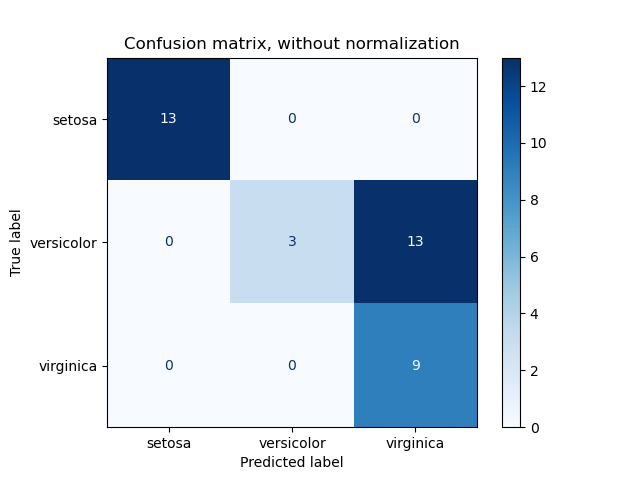
The parameter normalize allows to report ratios instead of counts. The
confusion matrix can be normalized in 3 different ways: 'pred', 'true',
and 'all' which will divide the counts by the sum of each columns, rows, or
the entire matrix, respectively.
>>> y_true = [0, 0, 0, 1, 1, 1, 1, 1]
>>> y_pred = [0, 1, 0, 1, 0, 1, 0, 1]
>>> confusion_matrix(y_true, y_pred, normalize='all')
array([[0.25 , 0.125],
       [0.25 , 0.375]])
For binary problems, we can get counts of true negatives, false positives,
false negatives and true positives as follows:
>>> y_true = [0, 0, 0, 1, 1, 1, 1, 1]
>>> y_pred = [0, 1, 0, 1, 0, 1, 0, 1]
>>> tn, fp, fn, tp = confusion_matrix(y_true, y_pred).ravel()
>>> tn, fp, fn, tp
(2, 1, 2, 3)
3.3.2.7. Classification report
The classification_report function builds a text report showing the
main classification metrics. Here is a small example with custom target_names
and inferred labels:
>>> from sklearn.metrics import classification_report
>>> y_true = [0, 1, 2, 2, 0]
>>> y_pred = [0, 0, 2, 1, 0]
>>> target_names = ['class 0', 'class 1', 'class 2']
>>> print(classification_report(y_true, y_pred, target_names=target_names))
              precision    recall  f1-score   support

     class 0       0.67      1.00      0.80         2
     class 1       0.00      0.00      0.00         1
     class 2       1.00      0.50      0.67         2

    accuracy                           0.60         5
   macro avg       0.56      0.50      0.49         5
weighted avg       0.67      0.60      0.59         5
3.3.2.8. Hamming loss
The hamming_loss computes the average Hamming loss or Hamming
distance between two sets
of samples.
If (hat{y}_{i,j}) is the predicted value for the (j)-th label of a
given sample (i), (y_{i,j}) is the corresponding true value,
(n_text{samples}) is the number of samples and (n_text{labels})
is the number of labels, then the Hamming loss (L_{Hamming}) is defined
as:
[L_{Hamming}(y, hat{y}) = frac{1}{n_text{samples} * n_text{labels}} sum_{i=0}^{n_text{samples}-1} sum_{j=0}^{n_text{labels} — 1} 1(hat{y}_{i,j} not= y_{i,j})]
where (1(x)) is the indicator function.
The equation above does not hold true in the case of multiclass classification.
Please refer to the note below for more information.
>>> from sklearn.metrics import hamming_loss
>>> y_pred = [1, 2, 3, 4]
>>> y_true = [2, 2, 3, 4]
>>> hamming_loss(y_true, y_pred)
0.25
In the multilabel case with binary label indicators:
>>> hamming_loss(np.array([[0, 1], [1, 1]]), np.zeros((2, 2)))
0.75
Note
In multiclass classification, the Hamming loss corresponds to the Hamming
distance between y_true and y_pred which is similar to the
Zero one loss function. However, while zero-one loss penalizes
prediction sets that do not strictly match true sets, the Hamming loss
penalizes individual labels. Thus the Hamming loss, upper bounded by the zero-one
loss, is always between zero and one, inclusive; and predicting a proper subset
or superset of the true labels will give a Hamming loss between
zero and one, exclusive.
3.3.2.9. Precision, recall and F-measures
Intuitively, precision is the ability
of the classifier not to label as positive a sample that is negative, and
recall is the
ability of the classifier to find all the positive samples.
The F-measure
((F_beta) and (F_1) measures) can be interpreted as a weighted
harmonic mean of the precision and recall. A
(F_beta) measure reaches its best value at 1 and its worst score at 0.
With (beta = 1), (F_beta) and
(F_1) are equivalent, and the recall and the precision are equally important.
The precision_recall_curve computes a precision-recall curve
from the ground truth label and a score given by the classifier
by varying a decision threshold.
The average_precision_score function computes the
average precision
(AP) from prediction scores. The value is between 0 and 1 and higher is better.
AP is defined as
[text{AP} = sum_n (R_n — R_{n-1}) P_n]
where (P_n) and (R_n) are the precision and recall at the
nth threshold. With random predictions, the AP is the fraction of positive
samples.
References [Manning2008] and [Everingham2010] present alternative variants of
AP that interpolate the precision-recall curve. Currently,
average_precision_score does not implement any interpolated variant.
References [Davis2006] and [Flach2015] describe why a linear interpolation of
points on the precision-recall curve provides an overly-optimistic measure of
classifier performance. This linear interpolation is used when computing area
under the curve with the trapezoidal rule in auc.
Several functions allow you to analyze the precision, recall and F-measures
score:
|
|
Compute average precision (AP) from prediction scores. |
|
|
Compute the F1 score, also known as balanced F-score or F-measure. |
|
|
Compute the F-beta score. |
|
|
Compute precision-recall pairs for different probability thresholds. |
|
|
Compute precision, recall, F-measure and support for each class. |
|
|
Compute the precision. |
|
|
Compute the recall. |
Note that the precision_recall_curve function is restricted to the
binary case. The average_precision_score function works only in
binary classification and multilabel indicator format.
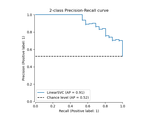
The PredictionRecallDisplay.from_estimator and
PredictionRecallDisplay.from_predictions functions will plot the
precision-recall curve as follows.
3.3.2.9.1. Binary classification
In a binary classification task, the terms ‘’positive’’ and ‘’negative’’ refer
to the classifier’s prediction, and the terms ‘’true’’ and ‘’false’’ refer to
whether that prediction corresponds to the external judgment (sometimes known
as the ‘’observation’’). Given these definitions, we can formulate the
following table:
|
Actual class (observation) |
||
|
Predicted class |
tp (true positive) |
fp (false positive) |
|
fn (false negative) |
tn (true negative) |
In this context, we can define the notions of precision, recall and F-measure:
[text{precision} = frac{tp}{tp + fp},]
[text{recall} = frac{tp}{tp + fn},]
[F_beta = (1 + beta^2) frac{text{precision} times text{recall}}{beta^2 text{precision} + text{recall}}.]
Sometimes recall is also called ‘’sensitivity’’.
Here are some small examples in binary classification:
>>> from sklearn import metrics
>>> y_pred = [0, 1, 0, 0]
>>> y_true = [0, 1, 0, 1]
>>> metrics.precision_score(y_true, y_pred)
1.0
>>> metrics.recall_score(y_true, y_pred)
0.5
>>> metrics.f1_score(y_true, y_pred)
0.66...
>>> metrics.fbeta_score(y_true, y_pred, beta=0.5)
0.83...
>>> metrics.fbeta_score(y_true, y_pred, beta=1)
0.66...
>>> metrics.fbeta_score(y_true, y_pred, beta=2)
0.55...
>>> metrics.precision_recall_fscore_support(y_true, y_pred, beta=0.5)
(array([0.66..., 1.        ]), array([1. , 0.5]), array([0.71..., 0.83...]), array([2, 2]))


>>> import numpy as np
>>> from sklearn.metrics import precision_recall_curve
>>> from sklearn.metrics import average_precision_score
>>> y_true = np.array([0, 0, 1, 1])
>>> y_scores = np.array([0.1, 0.4, 0.35, 0.8])
>>> precision, recall, threshold = precision_recall_curve(y_true, y_scores)
>>> precision
array([0.5       , 0.66..., 0.5       , 1.        , 1.        ])
>>> recall
array([1. , 1. , 0.5, 0.5, 0. ])
>>> threshold
array([0.1 , 0.35, 0.4 , 0.8 ])
>>> average_precision_score(y_true, y_scores)
0.83...
3.3.2.9.2. Multiclass and multilabel classification
In a multiclass and multilabel classification task, the notions of precision,
recall, and F-measures can be applied to each label independently.
There are a few ways to combine results across labels,
specified by the average argument to the
average_precision_score (multilabel only), f1_score,
fbeta_score, precision_recall_fscore_support,
precision_score and recall_score functions, as described
above. Note that if all labels are included, “micro”-averaging
in a multiclass setting will produce precision, recall and (F)
that are all identical to accuracy. Also note that “weighted” averaging may
produce an F-score that is not between precision and recall.
To make this more explicit, consider the following notation:
-
(y) the set of true ((sample, label)) pairs
-
(hat{y}) the set of predicted ((sample, label)) pairs
-
(L) the set of labels
-
(S) the set of samples
-
(y_s) the subset of (y) with sample (s),
i.e. (y_s := left{(s’, l) in y | s’ = sright}) -
(y_l) the subset of (y) with label (l)
-
similarly, (hat{y}_s) and (hat{y}_l) are subsets of
(hat{y}) -
(P(A, B) := frac{left| A cap B right|}{left|Bright|}) for some
sets (A) and (B) -
(R(A, B) := frac{left| A cap B right|}{left|Aright|})
(Conventions vary on handling (A = emptyset); this implementation uses
(R(A, B):=0), and similar for (P).) -
(F_beta(A, B) := left(1 + beta^2right) frac{P(A, B) times R(A, B)}{beta^2 P(A, B) + R(A, B)})
Then the metrics are defined as:
|
|
Precision |
Recall |
F_beta |
|---|---|---|---|
|
|
(P(y, hat{y})) |
(R(y, hat{y})) |
(F_beta(y, hat{y})) |
|
|
(frac{1}{left|Sright|} sum_{s in S} P(y_s, hat{y}_s)) |
(frac{1}{left|Sright|} sum_{s in S} R(y_s, hat{y}_s)) |
(frac{1}{left|Sright|} sum_{s in S} F_beta(y_s, hat{y}_s)) |
|
|
(frac{1}{left|Lright|} sum_{l in L} P(y_l, hat{y}_l)) |
(frac{1}{left|Lright|} sum_{l in L} R(y_l, hat{y}_l)) |
(frac{1}{left|Lright|} sum_{l in L} F_beta(y_l, hat{y}_l)) |
|
|
(frac{1}{sum_{l in L} left|y_lright|} sum_{l in L} left|y_lright| P(y_l, hat{y}_l)) |
(frac{1}{sum_{l in L} left|y_lright|} sum_{l in L} left|y_lright| R(y_l, hat{y}_l)) |
(frac{1}{sum_{l in L} left|y_lright|} sum_{l in L} left|y_lright| F_beta(y_l, hat{y}_l)) |
|
|
(langle P(y_l, hat{y}_l) | l in L rangle) |
(langle R(y_l, hat{y}_l) | l in L rangle) |
(langle F_beta(y_l, hat{y}_l) | l in L rangle) |
>>> from sklearn import metrics
>>> y_true = [0, 1, 2, 0, 1, 2]
>>> y_pred = [0, 2, 1, 0, 0, 1]
>>> metrics.precision_score(y_true, y_pred, average='macro')
0.22...
>>> metrics.recall_score(y_true, y_pred, average='micro')
0.33...
>>> metrics.f1_score(y_true, y_pred, average='weighted')
0.26...
>>> metrics.fbeta_score(y_true, y_pred, average='macro', beta=0.5)
0.23...
>>> metrics.precision_recall_fscore_support(y_true, y_pred, beta=0.5, average=None)
(array([0.66..., 0.        , 0.        ]), array([1., 0., 0.]), array([0.71..., 0.        , 0.        ]), array([2, 2, 2]...))
For multiclass classification with a “negative class”, it is possible to exclude some labels:
>>> metrics.recall_score(y_true, y_pred, labels=[1, 2], average='micro')
... # excluding 0, no labels were correctly recalled
0.0
Similarly, labels not present in the data sample may be accounted for in macro-averaging.
>>> metrics.precision_score(y_true, y_pred, labels=[0, 1, 2, 3], average='macro')
0.166...
3.3.2.10. Jaccard similarity coefficient score
The jaccard_score function computes the average of Jaccard similarity
coefficients, also called the
Jaccard index, between pairs of label sets.
The Jaccard similarity coefficient with a ground truth label set (y) and
predicted label set (hat{y}), is defined as
[J(y, hat{y}) = frac{|y cap hat{y}|}{|y cup hat{y}|}.]
The jaccard_score (like precision_recall_fscore_support) applies
natively to binary targets. By computing it set-wise it can be extended to apply
to multilabel and multiclass through the use of average (see
above).
In the binary case:
>>> import numpy as np
>>> from sklearn.metrics import jaccard_score
>>> y_true = np.array([[0, 1, 1],
...                    [1, 1, 0]])
>>> y_pred = np.array([[1, 1, 1],
...                    [1, 0, 0]])
>>> jaccard_score(y_true[0], y_pred[0])
0.6666...
In the 2D comparison case (e.g. image similarity):
>>> jaccard_score(y_true, y_pred, average="micro")
0.6
In the multilabel case with binary label indicators:
>>> jaccard_score(y_true, y_pred, average='samples')
0.5833...
>>> jaccard_score(y_true, y_pred, average='macro')
0.6666...
>>> jaccard_score(y_true, y_pred, average=None)
array([0.5, 0.5, 1. ])
Multiclass problems are binarized and treated like the corresponding
multilabel problem:
>>> y_pred = [0, 2, 1, 2]
>>> y_true = [0, 1, 2, 2]
>>> jaccard_score(y_true, y_pred, average=None)
array([1. , 0. , 0.33...])
>>> jaccard_score(y_true, y_pred, average='macro')
0.44...
>>> jaccard_score(y_true, y_pred, average='micro')
0.33...
3.3.2.11. Hinge loss
The hinge_loss function computes the average distance between
the model and the data using
hinge loss, a one-sided metric
that considers only prediction errors. (Hinge
loss is used in maximal margin classifiers such as support vector machines.)
If the true label (y_i) of a binary classification task is encoded as
(y_i=left{-1, +1right}) for every sample (i); and (w_i)
is the corresponding predicted decision (an array of shape (n_samples,) as
output by the decision_function method), then the hinge loss is defined as:
[L_text{Hinge}(y, w) = frac{1}{n_text{samples}} sum_{i=0}^{n_text{samples}-1} maxleft{1 — w_i y_i, 0right}]
If there are more than two labels, hinge_loss uses a multiclass variant
due to Crammer & Singer.
Here is
the paper describing it.
In this case the predicted decision is an array of shape (n_samples,
n_labels). If (w_{i, y_i}) is the predicted decision for the true label
(y_i) of the (i)-th sample; and
(hat{w}_{i, y_i} = maxleft{w_{i, y_j}~|~y_j ne y_i right})
is the maximum of the
predicted decisions for all the other labels, then the multi-class hinge loss
is defined by:
[L_text{Hinge}(y, w) = frac{1}{n_text{samples}}
sum_{i=0}^{n_text{samples}-1} maxleft{1 + hat{w}_{i, y_i}
— w_{i, y_i}, 0right}]
Here is a small example demonstrating the use of the hinge_loss function
with a svm classifier in a binary class problem:
>>> from sklearn import svm
>>> from sklearn.metrics import hinge_loss
>>> X = [[0], [1]]
>>> y = [-1, 1]
>>> est = svm.LinearSVC(random_state=0)
>>> est.fit(X, y)
LinearSVC(random_state=0)
>>> pred_decision = est.decision_function([[-2], [3], [0.5]])
>>> pred_decision
array([-2.18...,  2.36...,  0.09...])
>>> hinge_loss([-1, 1, 1], pred_decision)
0.3...
Here is an example demonstrating the use of the hinge_loss function
with a svm classifier in a multiclass problem:
>>> X = np.array([[0], [1], [2], [3]])
>>> Y = np.array([0, 1, 2, 3])
>>> labels = np.array([0, 1, 2, 3])
>>> est = svm.LinearSVC()
>>> est.fit(X, Y)
LinearSVC()
>>> pred_decision = est.decision_function([[-1], [2], [3]])
>>> y_true = [0, 2, 3]
>>> hinge_loss(y_true, pred_decision, labels=labels)
0.56...
3.3.2.12. Log loss
Log loss, also called logistic regression loss or
cross-entropy loss, is defined on probability estimates. It is
commonly used in (multinomial) logistic regression and neural networks, as well
as in some variants of expectation-maximization, and can be used to evaluate the
probability outputs (predict_proba) of a classifier instead of its
discrete predictions.
For binary classification with a true label (y in {0,1})
and a probability estimate (p = operatorname{Pr}(y = 1)),
the log loss per sample is the negative log-likelihood
of the classifier given the true label:
[L_{log}(y, p) = -log operatorname{Pr}(y|p) = -(y log (p) + (1 — y) log (1 — p))]
This extends to the multiclass case as follows.
Let the true labels for a set of samples
be encoded as a 1-of-K binary indicator matrix (Y),
i.e., (y_{i,k} = 1) if sample (i) has label (k)
taken from a set of (K) labels.
Let (P) be a matrix of probability estimates,
with (p_{i,k} = operatorname{Pr}(y_{i,k} = 1)).
Then the log loss of the whole set is
[L_{log}(Y, P) = -log operatorname{Pr}(Y|P) = — frac{1}{N} sum_{i=0}^{N-1} sum_{k=0}^{K-1} y_{i,k} log p_{i,k}]
To see how this generalizes the binary log loss given above,
note that in the binary case,
(p_{i,0} = 1 — p_{i,1}) and (y_{i,0} = 1 — y_{i,1}),
so expanding the inner sum over (y_{i,k} in {0,1})
gives the binary log loss.
The log_loss function computes log loss given a list of ground-truth
labels and a probability matrix, as returned by an estimator’s predict_proba
method.
>>> from sklearn.metrics import log_loss
>>> y_true = [0, 0, 1, 1]
>>> y_pred = [[.9, .1], [.8, .2], [.3, .7], [.01, .99]]
>>> log_loss(y_true, y_pred)
0.1738...
The first [.9, .1] in y_pred denotes 90% probability that the first
sample has label 0. The log loss is non-negative.
3.3.2.13. Matthews correlation coefficient
The matthews_corrcoef function computes the
Matthew’s correlation coefficient (MCC)
for binary classes. Quoting Wikipedia:
“The Matthews correlation coefficient is used in machine learning as a
measure of the quality of binary (two-class) classifications. It takes
into account true and false positives and negatives and is generally
regarded as a balanced measure which can be used even if the classes are
of very different sizes. The MCC is in essence a correlation coefficient
value between -1 and +1. A coefficient of +1 represents a perfect
prediction, 0 an average random prediction and -1 an inverse prediction.
The statistic is also known as the phi coefficient.”
In the binary (two-class) case, (tp), (tn), (fp) and
(fn) are respectively the number of true positives, true negatives, false
positives and false negatives, the MCC is defined as
[MCC = frac{tp times tn — fp times fn}{sqrt{(tp + fp)(tp + fn)(tn + fp)(tn + fn)}}.]
In the multiclass case, the Matthews correlation coefficient can be defined in terms of a
confusion_matrix (C) for (K) classes. To simplify the
definition consider the following intermediate variables:
-
(t_k=sum_{i}^{K} C_{ik}) the number of times class (k) truly occurred,
-
(p_k=sum_{i}^{K} C_{ki}) the number of times class (k) was predicted,
-
(c=sum_{k}^{K} C_{kk}) the total number of samples correctly predicted,
-
(s=sum_{i}^{K} sum_{j}^{K} C_{ij}) the total number of samples.
Then the multiclass MCC is defined as:
[MCC = frac{
c times s — sum_{k}^{K} p_k times t_k
}{sqrt{
(s^2 — sum_{k}^{K} p_k^2) times
(s^2 — sum_{k}^{K} t_k^2)
}}]
When there are more than two labels, the value of the MCC will no longer range
between -1 and +1. Instead the minimum value will be somewhere between -1 and 0
depending on the number and distribution of ground true labels. The maximum
value is always +1.
Here is a small example illustrating the usage of the matthews_corrcoef
function:
>>> from sklearn.metrics import matthews_corrcoef
>>> y_true = [+1, +1, +1, -1]
>>> y_pred = [+1, -1, +1, +1]
>>> matthews_corrcoef(y_true, y_pred)
-0.33...
3.3.2.14. Multi-label confusion matrix
The multilabel_confusion_matrix function computes class-wise (default)
or sample-wise (samplewise=True) multilabel confusion matrix to evaluate
the accuracy of a classification. multilabel_confusion_matrix also treats
multiclass data as if it were multilabel, as this is a transformation commonly
applied to evaluate multiclass problems with binary classification metrics
(such as precision, recall, etc.).
When calculating class-wise multilabel confusion matrix (C), the
count of true negatives for class (i) is (C_{i,0,0}), false
negatives is (C_{i,1,0}), true positives is (C_{i,1,1})
and false positives is (C_{i,0,1}).
Here is an example demonstrating the use of the
multilabel_confusion_matrix function with
multilabel indicator matrix input:
>>> import numpy as np
>>> from sklearn.metrics import multilabel_confusion_matrix
>>> y_true = np.array([[1, 0, 1],
...                    [0, 1, 0]])
>>> y_pred = np.array([[1, 0, 0],
...                    [0, 1, 1]])
>>> multilabel_confusion_matrix(y_true, y_pred)
array([[[1, 0],
        [0, 1]],

       [[1, 0],
        [0, 1]],

       [[0, 1],
        [1, 0]]])
Or a confusion matrix can be constructed for each sample’s labels:
>>> multilabel_confusion_matrix(y_true, y_pred, samplewise=True)
array([[[1, 0],
        [1, 1]],

       [[1, 1],
        [0, 1]]])
Here is an example demonstrating the use of the
multilabel_confusion_matrix function with
multiclass input:
>>> y_true = ["cat", "ant", "cat", "cat", "ant", "bird"]
>>> y_pred = ["ant", "ant", "cat", "cat", "ant", "cat"]
>>> multilabel_confusion_matrix(y_true, y_pred,
...                             labels=["ant", "bird", "cat"])
array([[[3, 1],
        [0, 2]],

       [[5, 0],
        [1, 0]],

       [[2, 1],
        [1, 2]]])
Here are some examples demonstrating the use of the
multilabel_confusion_matrix function to calculate recall
(or sensitivity), specificity, fall out and miss rate for each class in a
problem with multilabel indicator matrix input.
Calculating
recall
(also called the true positive rate or the sensitivity) for each class:
>>> y_true = np.array([[0, 0, 1],
...                    [0, 1, 0],
...                    [1, 1, 0]])
>>> y_pred = np.array([[0, 1, 0],
...                    [0, 0, 1],
...                    [1, 1, 0]])
>>> mcm = multilabel_confusion_matrix(y_true, y_pred)
>>> tn = mcm[:, 0, 0]
>>> tp = mcm[:, 1, 1]
>>> fn = mcm[:, 1, 0]
>>> fp = mcm[:, 0, 1]
>>> tp / (tp + fn)
array([1. , 0.5, 0. ])
Calculating
specificity
(also called the true negative rate) for each class:
>>> tn / (tn + fp)
array([1. , 0. , 0.5])
Calculating fall out
(also called the false positive rate) for each class:
>>> fp / (fp + tn)
array([0. , 1. , 0.5])
Calculating miss rate
(also called the false negative rate) for each class:
>>> fn / (fn + tp)
array([0. , 0.5, 1. ])
3.3.2.15. Receiver operating characteristic (ROC)
The function roc_curve computes the
receiver operating characteristic curve, or ROC curve.
Quoting Wikipedia :
“A receiver operating characteristic (ROC), or simply ROC curve, is a
graphical plot which illustrates the performance of a binary classifier
system as its discrimination threshold is varied. It is created by plotting
the fraction of true positives out of the positives (TPR = true positive
rate) vs. the fraction of false positives out of the negatives (FPR = false
positive rate), at various threshold settings. TPR is also known as
sensitivity, and FPR is one minus the specificity or true negative rate.”
This function requires the true binary value and the target scores, which can
either be probability estimates of the positive class, confidence values, or
binary decisions. Here is a small example of how to use the roc_curve
function:
>>> import numpy as np
>>> from sklearn.metrics import roc_curve
>>> y = np.array([1, 1, 2, 2])
>>> scores = np.array([0.1, 0.4, 0.35, 0.8])
>>> fpr, tpr, thresholds = roc_curve(y, scores, pos_label=2)
>>> fpr
array([0. , 0. , 0.5, 0.5, 1. ])
>>> tpr
array([0. , 0.5, 0.5, 1. , 1. ])
>>> thresholds
array([1.8 , 0.8 , 0.4 , 0.35, 0.1 ])
Compared to metrics such as the subset accuracy, the Hamming loss, or the
F1 score, ROC doesn’t require optimizing a threshold for each label.
The roc_auc_score function, denoted by ROC-AUC or AUROC, computes the
area under the ROC curve. By doing so, the curve information is summarized in
one number.
The following figure shows the ROC curve and ROC-AUC score for a classifier
aimed to distinguish the virginica flower from the rest of the species in the
Iris plants dataset:
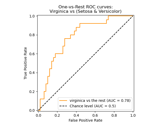
For more information see the Wikipedia article on AUC.
3.3.2.15.1. Binary case
In the binary case, you can either provide the probability estimates, using
the classifier.predict_proba() method, or the non-thresholded decision values
given by the classifier.decision_function() method. In the case of providing
the probability estimates, the probability of the class with the
“greater label” should be provided. The “greater label” corresponds to
classifier.classes_[1] and thus classifier.predict_proba(X)[:, 1].
Therefore, the y_score parameter is of size (n_samples,).
>>> from sklearn.datasets import load_breast_cancer
>>> from sklearn.linear_model import LogisticRegression
>>> from sklearn.metrics import roc_auc_score
>>> X, y = load_breast_cancer(return_X_y=True)
>>> clf = LogisticRegression(solver="liblinear").fit(X, y)
>>> clf.classes_
array([0, 1])
We can use the probability estimates corresponding to clf.classes_[1].
>>> y_score = clf.predict_proba(X)[:, 1]
>>> roc_auc_score(y, y_score)
0.99...
Otherwise, we can use the non-thresholded decision values
>>> roc_auc_score(y, clf.decision_function(X))
0.99...
3.3.2.15.2. Multi-class case
The roc_auc_score function can also be used in multi-class
classification. Two averaging strategies are currently supported: the
one-vs-one algorithm computes the average of the pairwise ROC AUC scores, and
the one-vs-rest algorithm computes the average of the ROC AUC scores for each
class against all other classes. In both cases, the predicted labels are
provided in an array with values from 0 to n_classes, and the scores
correspond to the probability estimates that a sample belongs to a particular
class. The OvO and OvR algorithms support weighting uniformly
(average='macro') and by prevalence (average='weighted').
One-vs-one Algorithm: Computes the average AUC of all possible pairwise
combinations of classes. [HT2001] defines a multiclass AUC metric weighted
uniformly:
[frac{1}{c(c-1)}sum_{j=1}^{c}sum_{k > j}^c (text{AUC}(j | k) +
text{AUC}(k | j))]
where (c) is the number of classes and (text{AUC}(j | k)) is the
AUC with class (j) as the positive class and class (k) as the
negative class. In general,
(text{AUC}(j | k) neq text{AUC}(k | j))) in the multiclass
case. This algorithm is used by setting the keyword argument multiclass
to 'ovo' and average to 'macro'.
The [HT2001] multiclass AUC metric can be extended to be weighted by the
prevalence:
[frac{1}{c(c-1)}sum_{j=1}^{c}sum_{k > j}^c p(j cup k)(
text{AUC}(j | k) + text{AUC}(k | j))]
where (c) is the number of classes. This algorithm is used by setting
the keyword argument multiclass to 'ovo' and average to
'weighted'. The 'weighted' option returns a prevalence-weighted average
as described in [FC2009].
One-vs-rest Algorithm: Computes the AUC of each class against the rest
[PD2000]. The algorithm is functionally the same as the multilabel case. To
enable this algorithm set the keyword argument multiclass to 'ovr'.
Additionally to 'macro' [F2006] and 'weighted' [F2001] averaging, OvR
supports 'micro' averaging.
In applications where a high false positive rate is not tolerable the parameter
max_fpr of roc_auc_score can be used to summarize the ROC curve up
to the given limit.
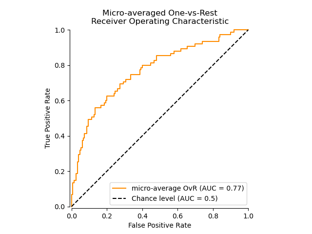
The following figure shows the micro-averaged ROC curve and its corresponding
ROC-AUC score for a classifier aimed to distinguish the the different species in
the Iris plants dataset:
3.3.2.15.3. Multi-label case
In multi-label classification, the roc_auc_score function is
extended by averaging over the labels as above. In this case,
you should provide a y_score of shape (n_samples, n_classes). Thus, when
using the probability estimates, one needs to select the probability of the
class with the greater label for each output.
>>> from sklearn.datasets import make_multilabel_classification
>>> from sklearn.multioutput import MultiOutputClassifier
>>> X, y = make_multilabel_classification(random_state=0)
>>> inner_clf = LogisticRegression(solver="liblinear", random_state=0)
>>> clf = MultiOutputClassifier(inner_clf).fit(X, y)
>>> y_score = np.transpose([y_pred[:, 1] for y_pred in clf.predict_proba(X)])
>>> roc_auc_score(y, y_score, average=None)
array([0.82..., 0.86..., 0.94..., 0.85... , 0.94...])
And the decision values do not require such processing.
>>> from sklearn.linear_model import RidgeClassifierCV
>>> clf = RidgeClassifierCV().fit(X, y)
>>> y_score = clf.decision_function(X)
>>> roc_auc_score(y, y_score, average=None)
array([0.81..., 0.84... , 0.93..., 0.87..., 0.94...])
3.3.2.16. Detection error tradeoff (DET)
The function det_curve computes the
detection error tradeoff curve (DET) curve [WikipediaDET2017].
Quoting Wikipedia:
“A detection error tradeoff (DET) graph is a graphical plot of error rates
for binary classification systems, plotting false reject rate vs. false
accept rate. The x- and y-axes are scaled non-linearly by their standard
normal deviates (or just by logarithmic transformation), yielding tradeoff
curves that are more linear than ROC curves, and use most of the image area
to highlight the differences of importance in the critical operating region.”
DET curves are a variation of receiver operating characteristic (ROC) curves
where False Negative Rate is plotted on the y-axis instead of True Positive
Rate.
DET curves are commonly plotted in normal deviate scale by transformation with
(phi^{-1}) (with (phi) being the cumulative distribution
function).
The resulting performance curves explicitly visualize the tradeoff of error
types for given classification algorithms.
See [Martin1997] for examples and further motivation.
This figure compares the ROC and DET curves of two example classifiers on the
same classification task:
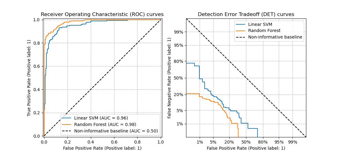
Properties:
-
DET curves form a linear curve in normal deviate scale if the detection
scores are normally (or close-to normally) distributed.
It was shown by [Navratil2007] that the reverse is not necessarily true and
even more general distributions are able to produce linear DET curves. -
The normal deviate scale transformation spreads out the points such that a
comparatively larger space of plot is occupied.
Therefore curves with similar classification performance might be easier to
distinguish on a DET plot. -
With False Negative Rate being “inverse” to True Positive Rate the point
of perfection for DET curves is the origin (in contrast to the top left
corner for ROC curves).
Applications and limitations:
DET curves are intuitive to read and hence allow quick visual assessment of a
classifier’s performance.
Additionally DET curves can be consulted for threshold analysis and operating
point selection.
This is particularly helpful if a comparison of error types is required.
On the other hand DET curves do not provide their metric as a single number.
Therefore for either automated evaluation or comparison to other
classification tasks metrics like the derived area under ROC curve might be
better suited.
3.3.2.17. Zero one loss
The zero_one_loss function computes the sum or the average of the 0-1
classification loss ((L_{0-1})) over (n_{text{samples}}). By
default, the function normalizes over the sample. To get the sum of the
(L_{0-1}), set normalize to False.
In multilabel classification, the zero_one_loss scores a subset as
one if its labels strictly match the predictions, and as a zero if there
are any errors. By default, the function returns the percentage of imperfectly
predicted subsets. To get the count of such subsets instead, set
normalize to False
If (hat{y}_i) is the predicted value of
the (i)-th sample and (y_i) is the corresponding true value,
then the 0-1 loss (L_{0-1}) is defined as:
[L_{0-1}(y, hat{y}) = frac{1}{n_text{samples}} sum_{i=0}^{n_text{samples}-1} 1(hat{y}_i not= y_i)]
where (1(x)) is the indicator function. The zero one
loss can also be computed as (zero-one loss = 1 — accuracy).
>>> from sklearn.metrics import zero_one_loss
>>> y_pred = [1, 2, 3, 4]
>>> y_true = [2, 2, 3, 4]
>>> zero_one_loss(y_true, y_pred)
0.25
>>> zero_one_loss(y_true, y_pred, normalize=False)
1
In the multilabel case with binary label indicators, where the first label
set [0,1] has an error:
>>> zero_one_loss(np.array([[0, 1], [1, 1]]), np.ones((2, 2)))
0.5

>>> zero_one_loss(np.array([[0, 1], [1, 1]]), np.ones((2, 2)),  normalize=False)
1
3.3.2.18. Brier score loss
The brier_score_loss function computes the
Brier score
for binary classes [Brier1950]. Quoting Wikipedia:
“The Brier score is a proper score function that measures the accuracy of
probabilistic predictions. It is applicable to tasks in which predictions
must assign probabilities to a set of mutually exclusive discrete outcomes.”
This function returns the mean squared error of the actual outcome
(y in {0,1}) and the predicted probability estimate
(p = operatorname{Pr}(y = 1)) (predict_proba) as outputted by:
[BS = frac{1}{n_{text{samples}}} sum_{i=0}^{n_{text{samples}} — 1}(y_i — p_i)^2]
The Brier score loss is also between 0 to 1 and the lower the value (the mean
square difference is smaller), the more accurate the prediction is.
Here is a small example of usage of this function:
>>> import numpy as np
>>> from sklearn.metrics import brier_score_loss
>>> y_true = np.array([0, 1, 1, 0])
>>> y_true_categorical = np.array(["spam", "ham", "ham", "spam"])
>>> y_prob = np.array([0.1, 0.9, 0.8, 0.4])
>>> y_pred = np.array([0, 1, 1, 0])
>>> brier_score_loss(y_true, y_prob)
0.055
>>> brier_score_loss(y_true, 1 - y_prob, pos_label=0)
0.055
>>> brier_score_loss(y_true_categorical, y_prob, pos_label="ham")
0.055
>>> brier_score_loss(y_true, y_prob > 0.5)
0.0
The Brier score can be used to assess how well a classifier is calibrated.
However, a lower Brier score loss does not always mean a better calibration.
This is because, by analogy with the bias-variance decomposition of the mean
squared error, the Brier score loss can be decomposed as the sum of calibration
loss and refinement loss [Bella2012]. Calibration loss is defined as the mean
squared deviation from empirical probabilities derived from the slope of ROC
segments. Refinement loss can be defined as the expected optimal loss as
measured by the area under the optimal cost curve. Refinement loss can change
independently from calibration loss, thus a lower Brier score loss does not
necessarily mean a better calibrated model. “Only when refinement loss remains
the same does a lower Brier score loss always mean better calibration”
[Bella2012], [Flach2008].
3.3.2.19. Class likelihood ratios
The class_likelihood_ratios function computes the positive and negative
likelihood ratios
(LR_pm) for binary classes, which can be interpreted as the ratio of
post-test to pre-test odds as explained below. As a consequence, this metric is
invariant w.r.t. the class prevalence (the number of samples in the positive
class divided by the total number of samples) and can be extrapolated between
populations regardless of any possible class imbalance.
The (LR_pm) metrics are therefore very useful in settings where the data
available to learn and evaluate a classifier is a study population with nearly
balanced classes, such as a case-control study, while the target application,
i.e. the general population, has very low prevalence.
The positive likelihood ratio (LR_+) is the probability of a classifier to
correctly predict that a sample belongs to the positive class divided by the
probability of predicting the positive class for a sample belonging to the
negative class:
[LR_+ = frac{text{PR}(P+|T+)}{text{PR}(P+|T-)}.]
The notation here refers to predicted ((P)) or true ((T)) label and
the sign (+) and (-) refer to the positive and negative class,
respectively, e.g. (P+) stands for “predicted positive”.
Analogously, the negative likelihood ratio (LR_-) is the probability of a
sample of the positive class being classified as belonging to the negative class
divided by the probability of a sample of the negative class being correctly
classified:
[LR_- = frac{text{PR}(P-|T+)}{text{PR}(P-|T-)}.]
For classifiers above chance (LR_+) above 1 higher is better, while
(LR_-) ranges from 0 to 1 and lower is better.
Values of (LR_pmapprox 1) correspond to chance level.
Notice that probabilities differ from counts, for instance
(operatorname{PR}(P+|T+)) is not equal to the number of true positive
counts tp (see the wikipedia page for
the actual formulas).
Interpretation across varying prevalence:
Both class likelihood ratios are interpretable in terms of an odds ratio
(pre-test and post-tests):
[text{post-test odds} = text{Likelihood ratio} times text{pre-test odds}.]
Odds are in general related to probabilities via
[text{odds} = frac{text{probability}}{1 — text{probability}},]
or equivalently
[text{probability} = frac{text{odds}}{1 + text{odds}}.]
On a given population, the pre-test probability is given by the prevalence. By
converting odds to probabilities, the likelihood ratios can be translated into a
probability of truly belonging to either class before and after a classifier
prediction:
[text{post-test odds} = text{Likelihood ratio} times
frac{text{pre-test probability}}{1 — text{pre-test probability}},]
[text{post-test probability} = frac{text{post-test odds}}{1 + text{post-test odds}}.]
Mathematical divergences:
The positive likelihood ratio is undefined when (fp = 0), which can be
interpreted as the classifier perfectly identifying positive cases. If (fp
= 0) and additionally (tp = 0), this leads to a zero/zero division. This
happens, for instance, when using a DummyClassifier that always predicts the
negative class and therefore the interpretation as a perfect classifier is lost.
The negative likelihood ratio is undefined when (tn = 0). Such divergence
is invalid, as (LR_- > 1) would indicate an increase in the odds of a
sample belonging to the positive class after being classified as negative, as if
the act of classifying caused the positive condition. This includes the case of
a DummyClassifier that always predicts the positive class (i.e. when
(tn=fn=0)).
Both class likelihood ratios are undefined when (tp=fn=0), which means
that no samples of the positive class were present in the testing set. This can
also happen when cross-validating highly imbalanced data.
In all the previous cases the class_likelihood_ratios function raises by
default an appropriate warning message and returns nan to avoid pollution when
averaging over cross-validation folds.
For a worked-out demonstration of the class_likelihood_ratios function,
see the example below.
3.3.3. Multilabel ranking metrics
In multilabel learning, each sample can have any number of ground truth labels
associated with it. The goal is to give high scores and better rank to
the ground truth labels.
3.3.3.1. Coverage error
The coverage_error function computes the average number of labels that
have to be included in the final prediction such that all true labels
are predicted. This is useful if you want to know how many top-scored-labels
you have to predict in average without missing any true one. The best value
of this metrics is thus the average number of true labels.
Note
Our implementation’s score is 1 greater than the one given in Tsoumakas
et al., 2010. This extends it to handle the degenerate case in which an
instance has 0 true labels.
Formally, given a binary indicator matrix of the ground truth labels
(y in left{0, 1right}^{n_text{samples} times n_text{labels}}) and the
score associated with each label
(hat{f} in mathbb{R}^{n_text{samples} times n_text{labels}}),
the coverage is defined as
[coverage(y, hat{f}) = frac{1}{n_{text{samples}}}
sum_{i=0}^{n_{text{samples}} — 1} max_{j:y_{ij} = 1} text{rank}_{ij}]
with (text{rank}_{ij} = left|left{k: hat{f}_{ik} geq hat{f}_{ij} right}right|).
Given the rank definition, ties in y_scores are broken by giving the
maximal rank that would have been assigned to all tied values.
Here is a small example of usage of this function:
>>> import numpy as np
>>> from sklearn.metrics import coverage_error
>>> y_true = np.array([[1, 0, 0], [0, 0, 1]])
>>> y_score = np.array([[0.75, 0.5, 1], [1, 0.2, 0.1]])
>>> coverage_error(y_true, y_score)
2.5
3.3.3.2. Label ranking average precision
The label_ranking_average_precision_score function
implements label ranking average precision (LRAP). This metric is linked to
the average_precision_score function, but is based on the notion of
label ranking instead of precision and recall.
Label ranking average precision (LRAP) averages over the samples the answer to
the following question: for each ground truth label, what fraction of
higher-ranked labels were true labels? This performance measure will be higher
if you are able to give better rank to the labels associated with each sample.
The obtained score is always strictly greater than 0, and the best value is 1.
If there is exactly one relevant label per sample, label ranking average
precision is equivalent to the mean
reciprocal rank.
Formally, given a binary indicator matrix of the ground truth labels
(y in left{0, 1right}^{n_text{samples} times n_text{labels}})
and the score associated with each label
(hat{f} in mathbb{R}^{n_text{samples} times n_text{labels}}),
the average precision is defined as
[LRAP(y, hat{f}) = frac{1}{n_{text{samples}}}
sum_{i=0}^{n_{text{samples}} — 1} frac{1}{||y_i||_0}
sum_{j:y_{ij} = 1} frac{|mathcal{L}_{ij}|}{text{rank}_{ij}}]
where
(mathcal{L}_{ij} = left{k: y_{ik} = 1, hat{f}_{ik} geq hat{f}_{ij} right}),
(text{rank}_{ij} = left|left{k: hat{f}_{ik} geq hat{f}_{ij} right}right|),
(|cdot|) computes the cardinality of the set (i.e., the number of
elements in the set), and (||cdot||_0) is the (ell_0) “norm”
(which computes the number of nonzero elements in a vector).
Here is a small example of usage of this function:
>>> import numpy as np
>>> from sklearn.metrics import label_ranking_average_precision_score
>>> y_true = np.array([[1, 0, 0], [0, 0, 1]])
>>> y_score = np.array([[0.75, 0.5, 1], [1, 0.2, 0.1]])
>>> label_ranking_average_precision_score(y_true, y_score)
0.416...
3.3.3.3. Ranking loss
The label_ranking_loss function computes the ranking loss which
averages over the samples the number of label pairs that are incorrectly
ordered, i.e. true labels have a lower score than false labels, weighted by
the inverse of the number of ordered pairs of false and true labels.
The lowest achievable ranking loss is zero.
Formally, given a binary indicator matrix of the ground truth labels
(y in left{0, 1right}^{n_text{samples} times n_text{labels}}) and the
score associated with each label
(hat{f} in mathbb{R}^{n_text{samples} times n_text{labels}}),
the ranking loss is defined as
[ranking_loss(y, hat{f}) = frac{1}{n_{text{samples}}}
sum_{i=0}^{n_{text{samples}} — 1} frac{1}{||y_i||_0(n_text{labels} — ||y_i||_0)}
left|left{(k, l): hat{f}_{ik} leq hat{f}_{il}, y_{ik} = 1, y_{il} = 0 right}right|]
where (|cdot|) computes the cardinality of the set (i.e., the number of
elements in the set) and (||cdot||_0) is the (ell_0) “norm”
(which computes the number of nonzero elements in a vector).
Here is a small example of usage of this function:
>>> import numpy as np
>>> from sklearn.metrics import label_ranking_loss
>>> y_true = np.array([[1, 0, 0], [0, 0, 1]])
>>> y_score = np.array([[0.75, 0.5, 1], [1, 0.2, 0.1]])
>>> label_ranking_loss(y_true, y_score)
0.75...
>>> # With the following prediction, we have perfect and minimal loss
>>> y_score = np.array([[1.0, 0.1, 0.2], [0.1, 0.2, 0.9]])
>>> label_ranking_loss(y_true, y_score)
0.0
3.3.3.4. Normalized Discounted Cumulative Gain
Discounted Cumulative Gain (DCG) and Normalized Discounted Cumulative Gain
(NDCG) are ranking metrics implemented in dcg_score
and ndcg_score ; they compare a predicted order to
ground-truth scores, such as the relevance of answers to a query.
From the Wikipedia page for Discounted Cumulative Gain:
“Discounted cumulative gain (DCG) is a measure of ranking quality. In
information retrieval, it is often used to measure effectiveness of web search
engine algorithms or related applications. Using a graded relevance scale of
documents in a search-engine result set, DCG measures the usefulness, or gain,
of a document based on its position in the result list. The gain is accumulated
from the top of the result list to the bottom, with the gain of each result
discounted at lower ranks”
DCG orders the true targets (e.g. relevance of query answers) in the predicted
order, then multiplies them by a logarithmic decay and sums the result. The sum
can be truncated after the first (K) results, in which case we call it
DCG@K.
NDCG, or NDCG@K is DCG divided by the DCG obtained by a perfect prediction, so
that it is always between 0 and 1. Usually, NDCG is preferred to DCG.
Compared with the ranking loss, NDCG can take into account relevance scores,
rather than a ground-truth ranking. So if the ground-truth consists only of an
ordering, the ranking loss should be preferred; if the ground-truth consists of
actual usefulness scores (e.g. 0 for irrelevant, 1 for relevant, 2 for very
relevant), NDCG can be used.
For one sample, given the vector of continuous ground-truth values for each
target (y in mathbb{R}^{M}), where (M) is the number of outputs, and
the prediction (hat{y}), which induces the ranking function (f), the
DCG score is
[sum_{r=1}^{min(K, M)}frac{y_{f(r)}}{log(1 + r)}]
and the NDCG score is the DCG score divided by the DCG score obtained for
(y).
3.3.4. Regression metrics
The sklearn.metrics module implements several loss, score, and utility
functions to measure regression performance. Some of those have been enhanced
to handle the multioutput case: mean_squared_error,
mean_absolute_error, r2_score,
explained_variance_score, mean_pinball_loss, d2_pinball_score
and d2_absolute_error_score.
These functions have a multioutput keyword argument which specifies the
way the scores or losses for each individual target should be averaged. The
default is 'uniform_average', which specifies a uniformly weighted mean
over outputs. If an ndarray of shape (n_outputs,) is passed, then its
entries are interpreted as weights and an according weighted average is
returned. If multioutput is 'raw_values', then all unaltered
individual scores or losses will be returned in an array of shape
(n_outputs,).
The r2_score and explained_variance_score accept an additional
value 'variance_weighted' for the multioutput parameter. This option
leads to a weighting of each individual score by the variance of the
corresponding target variable. This setting quantifies the globally captured
unscaled variance. If the target variables are of different scale, then this
score puts more importance on explaining the higher variance variables.
multioutput='variance_weighted' is the default value for r2_score
for backward compatibility. This will be changed to uniform_average in the
future.
3.3.4.1. R² score, the coefficient of determination
The r2_score function computes the coefficient of
determination,
usually denoted as (R^2).
It represents the proportion of variance (of y) that has been explained by the
independent variables in the model. It provides an indication of goodness of
fit and therefore a measure of how well unseen samples are likely to be
predicted by the model, through the proportion of explained variance.
As such variance is dataset dependent, (R^2) may not be meaningfully comparable
across different datasets. Best possible score is 1.0 and it can be negative
(because the model can be arbitrarily worse). A constant model that always
predicts the expected (average) value of y, disregarding the input features,
would get an (R^2) score of 0.0.
Note: when the prediction residuals have zero mean, the (R^2) score and
the Explained variance score are identical.
If (hat{y}_i) is the predicted value of the (i)-th sample
and (y_i) is the corresponding true value for total (n) samples,
the estimated (R^2) is defined as:
[R^2(y, hat{y}) = 1 — frac{sum_{i=1}^{n} (y_i — hat{y}_i)^2}{sum_{i=1}^{n} (y_i — bar{y})^2}]
where (bar{y} = frac{1}{n} sum_{i=1}^{n} y_i) and (sum_{i=1}^{n} (y_i — hat{y}_i)^2 = sum_{i=1}^{n} epsilon_i^2).
Note that r2_score calculates unadjusted (R^2) without correcting for
bias in sample variance of y.
In the particular case where the true target is constant, the (R^2) score is
not finite: it is either NaN (perfect predictions) or -Inf (imperfect
predictions). Such non-finite scores may prevent correct model optimization
such as grid-search cross-validation to be performed correctly. For this reason
the default behaviour of r2_score is to replace them with 1.0 (perfect
predictions) or 0.0 (imperfect predictions). If force_finite
is set to False, this score falls back on the original (R^2) definition.
Here is a small example of usage of the r2_score function:
>>> from sklearn.metrics import r2_score
>>> y_true = [3, -0.5, 2, 7]
>>> y_pred = [2.5, 0.0, 2, 8]
>>> r2_score(y_true, y_pred)
0.948...
>>> y_true = [[0.5, 1], [-1, 1], [7, -6]]
>>> y_pred = [[0, 2], [-1, 2], [8, -5]]
>>> r2_score(y_true, y_pred, multioutput='variance_weighted')
0.938...
>>> y_true = [[0.5, 1], [-1, 1], [7, -6]]
>>> y_pred = [[0, 2], [-1, 2], [8, -5]]
>>> r2_score(y_true, y_pred, multioutput='uniform_average')
0.936...
>>> r2_score(y_true, y_pred, multioutput='raw_values')
array([0.965..., 0.908...])
>>> r2_score(y_true, y_pred, multioutput=[0.3, 0.7])
0.925...
>>> y_true = [-2, -2, -2]
>>> y_pred = [-2, -2, -2]
>>> r2_score(y_true, y_pred)
1.0
>>> r2_score(y_true, y_pred, force_finite=False)
nan
>>> y_true = [-2, -2, -2]
>>> y_pred = [-2, -2, -2 + 1e-8]
>>> r2_score(y_true, y_pred)
0.0
>>> r2_score(y_true, y_pred, force_finite=False)
-inf
3.3.4.2. Mean absolute error
The mean_absolute_error function computes mean absolute
error, a risk
metric corresponding to the expected value of the absolute error loss or
(l1)-norm loss.
If (hat{y}_i) is the predicted value of the (i)-th sample,
and (y_i) is the corresponding true value, then the mean absolute error
(MAE) estimated over (n_{text{samples}}) is defined as
[text{MAE}(y, hat{y}) = frac{1}{n_{text{samples}}} sum_{i=0}^{n_{text{samples}}-1} left| y_i — hat{y}_i right|.]
Here is a small example of usage of the mean_absolute_error function:
>>> from sklearn.metrics import mean_absolute_error
>>> y_true = [3, -0.5, 2, 7]
>>> y_pred = [2.5, 0.0, 2, 8]
>>> mean_absolute_error(y_true, y_pred)
0.5
>>> y_true = [[0.5, 1], [-1, 1], [7, -6]]
>>> y_pred = [[0, 2], [-1, 2], [8, -5]]
>>> mean_absolute_error(y_true, y_pred)
0.75
>>> mean_absolute_error(y_true, y_pred, multioutput='raw_values')
array([0.5, 1. ])
>>> mean_absolute_error(y_true, y_pred, multioutput=[0.3, 0.7])
0.85...
3.3.4.3. Mean squared error
The mean_squared_error function computes mean square
error, a risk
metric corresponding to the expected value of the squared (quadratic) error or
loss.
If (hat{y}_i) is the predicted value of the (i)-th sample,
and (y_i) is the corresponding true value, then the mean squared error
(MSE) estimated over (n_{text{samples}}) is defined as
[text{MSE}(y, hat{y}) = frac{1}{n_text{samples}} sum_{i=0}^{n_text{samples} — 1} (y_i — hat{y}_i)^2.]
Here is a small example of usage of the mean_squared_error
function:
>>> from sklearn.metrics import mean_squared_error
>>> y_true = [3, -0.5, 2, 7]
>>> y_pred = [2.5, 0.0, 2, 8]
>>> mean_squared_error(y_true, y_pred)
0.375
>>> y_true = [[0.5, 1], [-1, 1], [7, -6]]
>>> y_pred = [[0, 2], [-1, 2], [8, -5]]
>>> mean_squared_error(y_true, y_pred)
0.7083...
3.3.4.4. Mean squared logarithmic error
The mean_squared_log_error function computes a risk metric
corresponding to the expected value of the squared logarithmic (quadratic)
error or loss.
If (hat{y}_i) is the predicted value of the (i)-th sample,
and (y_i) is the corresponding true value, then the mean squared
logarithmic error (MSLE) estimated over (n_{text{samples}}) is
defined as
[text{MSLE}(y, hat{y}) = frac{1}{n_text{samples}} sum_{i=0}^{n_text{samples} — 1} (log_e (1 + y_i) — log_e (1 + hat{y}_i) )^2.]
Where (log_e (x)) means the natural logarithm of (x). This metric
is best to use when targets having exponential growth, such as population
counts, average sales of a commodity over a span of years etc. Note that this
metric penalizes an under-predicted estimate greater than an over-predicted
estimate.
Here is a small example of usage of the mean_squared_log_error
function:
>>> from sklearn.metrics import mean_squared_log_error
>>> y_true = [3, 5, 2.5, 7]
>>> y_pred = [2.5, 5, 4, 8]
>>> mean_squared_log_error(y_true, y_pred)
0.039...
>>> y_true = [[0.5, 1], [1, 2], [7, 6]]
>>> y_pred = [[0.5, 2], [1, 2.5], [8, 8]]
>>> mean_squared_log_error(y_true, y_pred)
0.044...
3.3.4.5. Mean absolute percentage error
The mean_absolute_percentage_error (MAPE), also known as mean absolute
percentage deviation (MAPD), is an evaluation metric for regression problems.
The idea of this metric is to be sensitive to relative errors. It is for example
not changed by a global scaling of the target variable.
If (hat{y}_i) is the predicted value of the (i)-th sample
and (y_i) is the corresponding true value, then the mean absolute percentage
error (MAPE) estimated over (n_{text{samples}}) is defined as
[text{MAPE}(y, hat{y}) = frac{1}{n_{text{samples}}} sum_{i=0}^{n_{text{samples}}-1} frac{{}left| y_i — hat{y}_i right|}{max(epsilon, left| y_i right|)}]
where (epsilon) is an arbitrary small yet strictly positive number to
avoid undefined results when y is zero.
The mean_absolute_percentage_error function supports multioutput.
Here is a small example of usage of the mean_absolute_percentage_error
function:
>>> from sklearn.metrics import mean_absolute_percentage_error
>>> y_true = [1, 10, 1e6]
>>> y_pred = [0.9, 15, 1.2e6]
>>> mean_absolute_percentage_error(y_true, y_pred)
0.2666...
In above example, if we had used mean_absolute_error, it would have ignored
the small magnitude values and only reflected the error in prediction of highest
magnitude value. But that problem is resolved in case of MAPE because it calculates
relative percentage error with respect to actual output.
3.3.4.6. Median absolute error
The median_absolute_error is particularly interesting because it is
robust to outliers. The loss is calculated by taking the median of all absolute
differences between the target and the prediction.
If (hat{y}_i) is the predicted value of the (i)-th sample
and (y_i) is the corresponding true value, then the median absolute error
(MedAE) estimated over (n_{text{samples}}) is defined as
[text{MedAE}(y, hat{y}) = text{median}(mid y_1 — hat{y}_1 mid, ldots, mid y_n — hat{y}_n mid).]
The median_absolute_error does not support multioutput.
Here is a small example of usage of the median_absolute_error
function:
>>> from sklearn.metrics import median_absolute_error
>>> y_true = [3, -0.5, 2, 7]
>>> y_pred = [2.5, 0.0, 2, 8]
>>> median_absolute_error(y_true, y_pred)
0.5
3.3.4.7. Max error
The max_error function computes the maximum residual error , a metric
that captures the worst case error between the predicted value and
the true value. In a perfectly fitted single output regression
model, max_error would be 0 on the training set and though this
would be highly unlikely in the real world, this metric shows the
extent of error that the model had when it was fitted.
If (hat{y}_i) is the predicted value of the (i)-th sample,
and (y_i) is the corresponding true value, then the max error is
defined as
[text{Max Error}(y, hat{y}) = max(| y_i — hat{y}_i |)]
Here is a small example of usage of the max_error function:
>>> from sklearn.metrics import max_error
>>> y_true = [3, 2, 7, 1]
>>> y_pred = [9, 2, 7, 1]
>>> max_error(y_true, y_pred)
6
The max_error does not support multioutput.
3.3.4.8. Explained variance score
The explained_variance_score computes the explained variance
regression score.
If (hat{y}) is the estimated target output, (y) the corresponding
(correct) target output, and (Var) is Variance, the square of the standard deviation,
then the explained variance is estimated as follow:
[explained_{}variance(y, hat{y}) = 1 — frac{Var{ y — hat{y}}}{Var{y}}]
The best possible score is 1.0, lower values are worse.
In the particular case where the true target is constant, the Explained
Variance score is not finite: it is either NaN (perfect predictions) or
-Inf (imperfect predictions). Such non-finite scores may prevent correct
model optimization such as grid-search cross-validation to be performed
correctly. For this reason the default behaviour of
explained_variance_score is to replace them with 1.0 (perfect
predictions) or 0.0 (imperfect predictions). You can set the force_finite
parameter to False to prevent this fix from happening and fallback on the
original Explained Variance score.
Here is a small example of usage of the explained_variance_score
function:
>>> from sklearn.metrics import explained_variance_score
>>> y_true = [3, -0.5, 2, 7]
>>> y_pred = [2.5, 0.0, 2, 8]
>>> explained_variance_score(y_true, y_pred)
0.957...
>>> y_true = [[0.5, 1], [-1, 1], [7, -6]]
>>> y_pred = [[0, 2], [-1, 2], [8, -5]]
>>> explained_variance_score(y_true, y_pred, multioutput='raw_values')
array([0.967..., 1.        ])
>>> explained_variance_score(y_true, y_pred, multioutput=[0.3, 0.7])
0.990...
>>> y_true = [-2, -2, -2]
>>> y_pred = [-2, -2, -2]
>>> explained_variance_score(y_true, y_pred)
1.0
>>> explained_variance_score(y_true, y_pred, force_finite=False)
nan
>>> y_true = [-2, -2, -2]
>>> y_pred = [-2, -2, -2 + 1e-8]
>>> explained_variance_score(y_true, y_pred)
0.0
>>> explained_variance_score(y_true, y_pred, force_finite=False)
-inf
3.3.4.9. Mean Poisson, Gamma, and Tweedie deviances
The mean_tweedie_deviance function computes the mean Tweedie
deviance error
with a power parameter ((p)). This is a metric that elicits
predicted expectation values of regression targets.
Following special cases exist,
-
when
power=0it is equivalent tomean_squared_error. -
when
power=1it is equivalent tomean_poisson_deviance. -
when
power=2it is equivalent tomean_gamma_deviance.
If (hat{y}_i) is the predicted value of the (i)-th sample,
and (y_i) is the corresponding true value, then the mean Tweedie
deviance error (D) for power (p), estimated over (n_{text{samples}})
is defined as
[begin{split}text{D}(y, hat{y}) = frac{1}{n_text{samples}}
sum_{i=0}^{n_text{samples} — 1}
begin{cases}
(y_i-hat{y}_i)^2, & text{for }p=0text{ (Normal)}\
2(y_i log(y_i/hat{y}_i) + hat{y}_i — y_i), & text{for }p=1text{ (Poisson)}\
2(log(hat{y}_i/y_i) + y_i/hat{y}_i — 1), & text{for }p=2text{ (Gamma)}\
2left(frac{max(y_i,0)^{2-p}}{(1-p)(2-p)}-
frac{y_i,hat{y}_i^{1-p}}{1-p}+frac{hat{y}_i^{2-p}}{2-p}right),
& text{otherwise}
end{cases}end{split}]
Tweedie deviance is a homogeneous function of degree 2-power.
Thus, Gamma distribution with power=2 means that simultaneously scaling
y_true and y_pred has no effect on the deviance. For Poisson
distribution power=1 the deviance scales linearly, and for Normal
distribution (power=0), quadratically. In general, the higher
power the less weight is given to extreme deviations between true
and predicted targets.
For instance, let’s compare the two predictions 1.5 and 150 that are both
50% larger than their corresponding true value.
The mean squared error (power=0) is very sensitive to the
prediction difference of the second point,:
>>> from sklearn.metrics import mean_tweedie_deviance
>>> mean_tweedie_deviance([1.0], [1.5], power=0)
0.25
>>> mean_tweedie_deviance([100.], [150.], power=0)
2500.0
If we increase power to 1,:
>>> mean_tweedie_deviance([1.0], [1.5], power=1)
0.18...
>>> mean_tweedie_deviance([100.], [150.], power=1)
18.9...
the difference in errors decreases. Finally, by setting, power=2:
>>> mean_tweedie_deviance([1.0], [1.5], power=2)
0.14...
>>> mean_tweedie_deviance([100.], [150.], power=2)
0.14...
we would get identical errors. The deviance when power=2 is thus only
sensitive to relative errors.
3.3.4.10. Pinball loss
The mean_pinball_loss function is used to evaluate the predictive
performance of quantile regression models.
[text{pinball}(y, hat{y}) = frac{1}{n_{text{samples}}} sum_{i=0}^{n_{text{samples}}-1} alpha max(y_i — hat{y}_i, 0) + (1 — alpha) max(hat{y}_i — y_i, 0)]
The value of pinball loss is equivalent to half of mean_absolute_error when the quantile
parameter alpha is set to 0.5.
Here is a small example of usage of the mean_pinball_loss function:
>>> from sklearn.metrics import mean_pinball_loss
>>> y_true = [1, 2, 3]
>>> mean_pinball_loss(y_true, [0, 2, 3], alpha=0.1)
0.03...
>>> mean_pinball_loss(y_true, [1, 2, 4], alpha=0.1)
0.3...
>>> mean_pinball_loss(y_true, [0, 2, 3], alpha=0.9)
0.3...
>>> mean_pinball_loss(y_true, [1, 2, 4], alpha=0.9)
0.03...
>>> mean_pinball_loss(y_true, y_true, alpha=0.1)
0.0
>>> mean_pinball_loss(y_true, y_true, alpha=0.9)
0.0
It is possible to build a scorer object with a specific choice of alpha:
>>> from sklearn.metrics import make_scorer
>>> mean_pinball_loss_95p = make_scorer(mean_pinball_loss, alpha=0.95)
Such a scorer can be used to evaluate the generalization performance of a
quantile regressor via cross-validation:
>>> from sklearn.datasets import make_regression
>>> from sklearn.model_selection import cross_val_score
>>> from sklearn.ensemble import GradientBoostingRegressor
>>>
>>> X, y = make_regression(n_samples=100, random_state=0)
>>> estimator = GradientBoostingRegressor(
...     loss="quantile",
...     alpha=0.95,
...     random_state=0,
... )
>>> cross_val_score(estimator, X, y, cv=5, scoring=mean_pinball_loss_95p)
array([13.6..., 9.7..., 23.3..., 9.5..., 10.4...])
It is also possible to build scorer objects for hyper-parameter tuning. The
sign of the loss must be switched to ensure that greater means better as
explained in the example linked below.
3.3.4.11. D² score
The D² score computes the fraction of deviance explained.
It is a generalization of R², where the squared error is generalized and replaced
by a deviance of choice (text{dev}(y, hat{y}))
(e.g., Tweedie, pinball or mean absolute error). D² is a form of a skill score.
It is calculated as
[D^2(y, hat{y}) = 1 — frac{text{dev}(y, hat{y})}{text{dev}(y, y_{text{null}})} ,.]
Where (y_{text{null}}) is the optimal prediction of an intercept-only model
(e.g., the mean of y_true for the Tweedie case, the median for absolute
error and the alpha-quantile for pinball loss).
Like R², the best possible score is 1.0 and it can be negative (because the
model can be arbitrarily worse). A constant model that always predicts
(y_{text{null}}), disregarding the input features, would get a D² score
of 0.0.
3.3.4.11.1. D² Tweedie score
The d2_tweedie_score function implements the special case of D²
where (text{dev}(y, hat{y})) is the Tweedie deviance, see Mean Poisson, Gamma, and Tweedie deviances.
It is also known as D² Tweedie and is related to McFadden’s likelihood ratio index.
The argument power defines the Tweedie power as for
mean_tweedie_deviance. Note that for power=0,
d2_tweedie_score equals r2_score (for single targets).
A scorer object with a specific choice of power can be built by:
>>> from sklearn.metrics import d2_tweedie_score, make_scorer
>>> d2_tweedie_score_15 = make_scorer(d2_tweedie_score, power=1.5)
3.3.4.11.2. D² pinball score
The d2_pinball_score function implements the special case
of D² with the pinball loss, see Pinball loss, i.e.:
[text{dev}(y, hat{y}) = text{pinball}(y, hat{y}).]
The argument alpha defines the slope of the pinball loss as for
mean_pinball_loss (Pinball loss). It determines the
quantile level alpha for which the pinball loss and also D²
are optimal. Note that for alpha=0.5 (the default) d2_pinball_score
equals d2_absolute_error_score.
A scorer object with a specific choice of alpha can be built by:
>>> from sklearn.metrics import d2_pinball_score, make_scorer
>>> d2_pinball_score_08 = make_scorer(d2_pinball_score, alpha=0.8)
3.3.4.11.3. D² absolute error score
The d2_absolute_error_score function implements the special case of
the Mean absolute error:
[text{dev}(y, hat{y}) = text{MAE}(y, hat{y}).]
Here are some usage examples of the d2_absolute_error_score function:
>>> from sklearn.metrics import d2_absolute_error_score
>>> y_true = [3, -0.5, 2, 7]
>>> y_pred = [2.5, 0.0, 2, 8]
>>> d2_absolute_error_score(y_true, y_pred)
0.764...
>>> y_true = [1, 2, 3]
>>> y_pred = [1, 2, 3]
>>> d2_absolute_error_score(y_true, y_pred)
1.0
>>> y_true = [1, 2, 3]
>>> y_pred = [2, 2, 2]
>>> d2_absolute_error_score(y_true, y_pred)
0.0
3.3.4.12. Visual evaluation of regression models
Among methods to assess the quality of regression models, scikit-learn provides
the PredictionErrorDisplay class. It allows to
visually inspect the prediction errors of a model in two different manners.
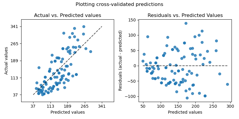
The plot on the left shows the actual values vs predicted values. For a
noise-free regression task aiming to predict the (conditional) expectation of
y, a perfect regression model would display data points on the diagonal
defined by predicted equal to actual values. The further away from this optimal
line, the larger the error of the model. In a more realistic setting with
irreducible noise, that is, when not all the variations of y can be explained
by features in X, then the best model would lead to a cloud of points densely
arranged around the diagonal.
Note that the above only holds when the predicted values is the expected value
of y given X. This is typically the case for regression models that
minimize the mean squared error objective function or more generally the
mean Tweedie deviance for any value of its
“power” parameter.
When plotting the predictions of an estimator that predicts a quantile
of y given X, e.g. QuantileRegressor
or any other model minimizing the pinball loss, a
fraction of the points are either expected to lie above or below the diagonal
depending on the estimated quantile level.
All in all, while intuitive to read, this plot does not really inform us on
what to do to obtain a better model.
The right-hand side plot shows the residuals (i.e. the difference between the
actual and the predicted values) vs. the predicted values.
This plot makes it easier to visualize if the residuals follow and
homoscedastic or heteroschedastic
distribution.
In particular, if the true distribution of y|X is Poisson or Gamma
distributed, it is expected that the variance of the residuals of the optimal
model would grow with the predicted value of E[y|X] (either linearly for
Poisson or quadratically for Gamma).
When fitting a linear least squares regression model (see
LinearRegression and
Ridge), we can use this plot to check
if some of the model assumptions
are met, in particular that the residuals should be uncorrelated, their
expected value should be null and that their variance should be constant
(homoschedasticity).
If this is not the case, and in particular if the residuals plot show some
banana-shaped structure, this is a hint that the model is likely mis-specified
and that non-linear feature engineering or switching to a non-linear regression
model might be useful.
Refer to the example below to see a model evaluation that makes use of this
display.
3.3.5. Clustering metrics
The sklearn.metrics module implements several loss, score, and utility
functions. For more information see the Clustering performance evaluation
section for instance clustering, and Biclustering evaluation for
biclustering.
3.3.6. Dummy estimators
When doing supervised learning, a simple sanity check consists of comparing
one’s estimator against simple rules of thumb. DummyClassifier
implements several such simple strategies for classification:
-
stratifiedgenerates random predictions by respecting the training
set class distribution. -
most_frequentalways predicts the most frequent label in the training set. -
prioralways predicts the class that maximizes the class prior
(likemost_frequent) andpredict_probareturns the class prior. -
uniformgenerates predictions uniformly at random. -
constantalways predicts a constant label that is provided by the user.-
A major motivation of this method is F1-scoring, when the positive class
is in the minority.
Note that with all these strategies, the predict method completely ignores
the input data!
To illustrate DummyClassifier, first let’s create an imbalanced
dataset:
>>> from sklearn.datasets import load_iris
>>> from sklearn.model_selection import train_test_split
>>> X, y = load_iris(return_X_y=True)
>>> y[y != 1] = -1
>>> X_train, X_test, y_train, y_test = train_test_split(X, y, random_state=0)
Next, let’s compare the accuracy of SVC and most_frequent:
>>> from sklearn.dummy import DummyClassifier
>>> from sklearn.svm import SVC
>>> clf = SVC(kernel='linear', C=1).fit(X_train, y_train)
>>> clf.score(X_test, y_test)
0.63...
>>> clf = DummyClassifier(strategy='most_frequent', random_state=0)
>>> clf.fit(X_train, y_train)
DummyClassifier(random_state=0, strategy='most_frequent')
>>> clf.score(X_test, y_test)
0.57...
We see that SVC doesn’t do much better than a dummy classifier. Now, let’s
change the kernel:
>>> clf = SVC(kernel='rbf', C=1).fit(X_train, y_train)
>>> clf.score(X_test, y_test)
0.94...
We see that the accuracy was boosted to almost 100%. A cross validation
strategy is recommended for a better estimate of the accuracy, if it
is not too CPU costly. For more information see the Cross-validation: evaluating estimator performance
section. Moreover if you want to optimize over the parameter space, it is highly
recommended to use an appropriate methodology; see the Tuning the hyper-parameters of an estimator
section for details.
More generally, when the accuracy of a classifier is too close to random, it
probably means that something went wrong: features are not helpful, a
hyperparameter is not correctly tuned, the classifier is suffering from class
imbalance, etc…
DummyRegressor also implements four simple rules of thumb for regression:
-
meanalways predicts the mean of the training targets. -
medianalways predicts the median of the training targets. -
quantilealways predicts a user provided quantile of the training targets. -
constantalways predicts a constant value that is provided by the user.
In all these strategies, the predict method completely ignores
the input data.
| title | date | categories | tags | |||||
|---|---|---|---|---|---|---|---|---|
|
How to create a confusion matrix with Scikit-learn? |
2020-05-05 |
frameworks |
|
After training a supervised machine learning model such as a classifier, you would like to know how well it works.
This is often done by setting apart a small piece of your data called the test set, which is used as data that the model has never seen before.
If it performs well on this dataset, it is likely that the model performs well on other data too — if it is sampled from the same distribution as your test set, of course.
Now, when you test your model, you feed it the data — and compare the predictions with the ground truth, measuring the number of true positives, true negatives, false positives and false negatives. These can subsequently be visualized in a visually appealing confusion matrix.
In today’s blog post, we’ll show you how to create such a confusion matrix with Scikit-learn, one of the most widely used frameworks for machine learning in today’s ML community. By means of an example created with Python, we’ll show you step-by-step how to generate a matrix with which you can visually determine the performance of your model easily.
All right, let’s go! 
[toc]
A confusion matrix in more detail
Training your machine learning model involves its evaluation. In many cases, you have set apart a test set for this.
The test set is a dataset that the trained model has never seen before. Using it allows you to test whether the model has overfit, or adapted to the training data too well, or whether it still generalizes to new data.
This allows you to ensure that your model does not perform very poorly on new data while it still performs really good on the training set. That wouldn’t really work in practice, would it
Evaluation with a test set often happens by feeding all the samples to the model, generating a prediction. Subsequently, the predictions are compared with the ground truth — or the true targets corresponding to the test set. These can subsequently be used for computing various metrics.
But they can also be used to demonstrate model performance in a visual way.
Here is an example of a confusion matrix:

To be more precise, it is a normalized confusion matrix. Its axes describe two measures:
- The true labels, which are the ground truth represented by your test set.
- The predicted labels, which are the predictions generated by the machine learning model for the features corresponding to the true labels.
It allows you to easily compare how well your model performs. For example, in the model above, for all true labels 1, the predicted label is 1. This means that all samples from class 1 were classified correctly. Great!
For the other classes, performance is also good, but a little bit worse. As you can see, for class 2, some samples were predicted as being part of classes 0 and 1.
In short, it answers the question «For my true labels / ground truth, how well does the model predict?».
It’s also possible to start from a prediction point of view. In this case, the question would change to «For my predicted label, how many predictions are actually part of the predicted class?». It’s the opposite point of view, but could be a valid question in many machine learning cases.
Most preferably, the entire set of true labels is equal to the set of predicted labels. In those cases, you would see zeros everywhere except for the line from the top left to the bottom right. In practice, however, this does not happen often. Likely, the plot is much more scattered, like this SVM classifier where many supporrt vectors are necessary to draw a decision boundary that does not work perfectly, but adequately enough:


Creating a confusion matrix with Python and Scikit-learn
Let’s now see if we can create a confusion matrix ourselves. Today, we will be using Python and Scikit-learn, one of the most widely used frameworks for machine learning today.
Creating a confusion matrix involves various steps:
- Generating an example dataset. This one makes sense: we need data to train our model on. We’ll therefore be generating data first, so that we can make an adequate choice for a ML model class next.
- Picking a machine learning model class. Obviously, if we want to evaluate a model, we need to train a model. We’ll choose a particular type of model first that fits the characteristics of our data.
- Constructing and training the ML model. The consequence of the first two steps is that we end up with a trained model.
- Generating the confusion matrix. Finally, based on the trained model, we can create our confusion matrix.
Software dependencies you need to install
Very briefly, but importantly: if you wish to run this code, you must make sure that you have certain software dependencies installed. Here they are:
- You need to install Python, which is the platform that our code runs on, version 3.6+.
- You need to install Scikit-learn, the machine learning framework that we will be using today:
pip install -U scikit-learn. - You need to install Numpy for numbers processing:
pip install numpy. - You need to install Matplotlib for visualizing the plots:
pip install matplotlib. - Finally, if you wish to generate a plot of decision boundaries (not required), you also need to install Mlxtend:
pip install mlxtend.
[affiliatebox]
Generating an example dataset
The first step is generating an example dataset. We will be using Scikit-learn for this purpose too. First, create a file called confusion-matrix.py, and open it in a code editor. The first thing we do is add the imports:
# Imports
from sklearn.datasets import make_blobs
from sklearn.model_selection import train_test_split
import numpy as np
import matplotlib.pyplot as plt
The make_blobs function from Scikit-learn allows us to generate ‘blobs’, or clusters, of samples. Those blobs are centered around some point and are the samples are scattered around this point based on some standard deviation. This gives you flexibility about both the position and the structure of your generated dataset, in turn allowing you to experiment with a variety of ML models without having to worry about the data.
As we will evaluate the model, we need to ensure that the dataset is split between training and testing data. Scikit-learn also allows us to do this, with train_test_split. We therefore import that one too.
Configuration options
Next, we can define a number of configuration options:
# Configuration options
blobs_random_seed = 42
centers = [(0,0), (5,5), (0,5), (2,3)]
cluster_std = 1.3
frac_test_split = 0.33
num_features_for_samples = 4
num_samples_total = 5000
The random seed describes the initialization of the pseudo-random number generator used for generating the blobs of data. As you may know, no random number generator is truly random. What’s more, they are also initialized differently. Configuring a fixed seed ensures that every time you run the script, the random number generator initializes in the same way. If weird behavior occurs, you know that it’s likely not the random number generator.
The centers describe the centers in two-dimensional space of our blobs of data. As you can see, we have 4 blobs today.
The cluster standard deviation describes the standard deviation with which a sample is drawn from the sampling distribution used by the random point generator. We set it to 1.3; a lower number produces clusters that are better separable, and vice-versa.
The fraction of the train/test split determines how much data is split off for testing purposes. In our case, that’s 33% of the data.
The number of features for our samples is 4, and indeed describes how many targets we have: 4, as we have 4 blobs of data.
Finally, the number of samples generated is pretty self-explanatory. We set it to 5000 samples. That’s not too much data, but more than sufficient for the educational purposes of today’s blog post.
Generating the data
Next up is the call to make_blobs and to train_test_split for actually generating and splitting the data:
# Generate data
inputs, targets = make_blobs(n_samples = num_samples_total, centers = centers, n_features = num_features_for_samples, cluster_std = cluster_std)
X_train, X_test, y_train, y_test = train_test_split(inputs, targets, test_size=frac_test_split, random_state=blobs_random_seed)
Saving the data (optional)
Once the data is generated, you may choose to save it to file. This is an optional step — and I include it because I want to re-use the same dataset every time I run the script (e.g. because I am tweaking a visualization). If you use the code below, you can run it once — then, it’s saved in the .npy file. When you subsequently uncomment the np.save call, and possibly also the generate data calls, you’ll always have the same data load from file.
Then, you can tweak away your visualization easily without having to deal with new data all the time
# Save and load temporarily
np.save('./data_cf.npy', (X_train, X_test, y_train, y_test))
X_train, X_test, y_train, y_test = np.load('./data_cf.npy', allow_pickle=True)
Should you wish to visualize the data, this is of course possible:
# Generate scatter plot for training data
plt.scatter(X_train[:,0], X_train[:,1])
plt.title('Linearly separable data')
plt.xlabel('X1')
plt.ylabel('X2')
plt.show()
Picking a machine learning model class
Now that we have our code for generating the dataset, we can take a look at the output to determine what kind of model we could use:

I can derive a few characteristics from this dataset (which, obviously, I also built-in up front  ).
).
First of all, the number of features is low: only two — as our data is two-dimensional. This is good, because then we likely don’t face the curse of dimensionality, and a wider range of ML models is applicable.
Next, when inspecting the data from a closer point of view, I can see a gap between what seem to be blobs of data (it is also slightly visible in the diagram above):

This suggests that the data may be separable, and possibly even linearly so (yes, of course, I know this is the case ).
Third, and finally, the number of samples is relatively low: only 5.000 samples are present. Neural networks with their relatively large amount of trainable parameters would likely start overfitting relatively quickly, so they wouldn’t be my preferable choice.
However, traditional machine learning techniques to the rescue. A Support Vector Machine, which attempts to construct a decision boundary between separable blobs of data, can be a good candidate here. Let’s give it a try: we’re going to construct and train an SVM and see how well it performs through its confusion matrix.
Constructing and training the ML model
As we have seen in the post linked above, we can also use Scikit-learn to construct and train a SVM classifier. Let’s do so next.
Model imports
First, we’ll have to add a few extra imports to the top of our script:
from sklearn import svm
from sklearn.metrics import plot_confusion_matrix
from mlxtend.plotting import plot_decision_regions
(The Mlxtend one is optional, as we discussed at ‘what you need to install’, but could be useful if you wish to visualize the decision boundary later.)
Training the classifier
First, we initialize the SVM classifier. I’m using a linear kernel because I suspect (actually, I’m confident, as we constructed the data ourselves) that the data is linearly separable:
# Initialize SVM classifier
clf = svm.SVC(kernel='linear')
Then, we fit the training data — starting the training process:
# Fit data
clf = clf.fit(X_train, y_train)
That’s it for training the machine learning model! The classifier variable, or clf, now contains a reference to the trained classifier. By calling clf.predict, you can now generate predictions for new data.
Generating the confusion matrix
But let’s take a look at generating that confusion matrix now. As we discussed, it’s part of the evaluation step, and we use it to visualize its predictive and generalization power on the test set.
Recall that we compare the predictions generated during evaluation with the ground truth available for those inputs.
The plot_confusion_matrix call takes care of this for us, and we simply have to provide it the classifier (clf), the test set (X_test and y_test), a color map and whether to normalize the data.
# Generate confusion matrix
matrix = plot_confusion_matrix(clf, X_test, y_test,
                                 cmap=plt.cm.Blues,
                                 normalize='true')
plt.title('Confusion matrix for our classifier')
plt.show(matrix)
plt.show()

Normalization, here, involves converting back the data into the [0, 1] format above. If you leave out normalization, you get the number of samples that are part of that prediction:

Here are some other visualizations that help us explain the confusion matrix (for the boundary plot, you need to install Mlxtend with pip install mlxtend):


# Get support vectors
support_vectors = clf.support_vectors_

# Visualize support vectors
plt.scatter(X_train[:,0], X_train[:,1])
plt.scatter(support_vectors[:,0], support_vectors[:,1], color='red')
plt.title('Linearly separable data with support vectors')
plt.xlabel('X1')
plt.ylabel('X2')
plt.show()

# Plot decision boundary
plot_decision_regions(X_test, y_test, clf=clf, legend=2)
plt.show()
It’s clear that we need many support vectors (the red samples) to generate the decision boundary. Given the relative unclarity of the separability between the data points, this is not unexpected. I’m actually quite satisfied with the performance of the model, as demonstrated by the confusion matrix (relatively blue diagonal line).
The only class that underperforms is class 3, with a score of 0.68. It’s still acceptable, but is lower than preferred. This can be explained by looking at the class in the decision boundary plot. Here, it’s clear that it’s the middle class — the reds. As those samples are surrounded by the other ones, it’s clear that the model has had significant difficulty generating the decision boundary. We might for example counter this by using a different kernel function which takes this into account, ensuring better separability. However, that’s not the core of today’s post.
Full model code
Should you wish to obtain the full model code, that’s of course possible. Here you go
# Imports
from sklearn.datasets import make_blobs
from sklearn.model_selection import train_test_split
import numpy as np
import matplotlib.pyplot as plt
from sklearn import svm
from sklearn.metrics import plot_confusion_matrix
from mlxtend.plotting import plot_decision_regions

# Configuration options
blobs_random_seed = 42
centers = [(0,0), (5,5), (0,5), (2,3)]
cluster_std = 1.3
frac_test_split = 0.33
num_features_for_samples = 4
num_samples_total = 5000

# Generate data
inputs, targets = make_blobs(n_samples = num_samples_total, centers = centers, n_features = num_features_for_samples, cluster_std = cluster_std)
X_train, X_test, y_train, y_test = train_test_split(inputs, targets, test_size=frac_test_split, random_state=blobs_random_seed)

# Save and load temporarily
np.save('./data_cf.npy', (X_train, X_test, y_train, y_test))
X_train, X_test, y_train, y_test = np.load('./data_cf.npy', allow_pickle=True)

# Generate scatter plot for training data
plt.scatter(X_train[:,0], X_train[:,1])
plt.title('Linearly separable data')
plt.xlabel('X1')
plt.ylabel('X2')
plt.show()

# Initialize SVM classifier
clf = svm.SVC(kernel='linear')

# Fit data
clf = clf.fit(X_train, y_train)

# Generate confusion matrix
matrix = plot_confusion_matrix(clf, X_test, y_test,
                                 cmap=plt.cm.Blues)
plt.title('Confusion matrix for our classifier')
plt.show(matrix)
plt.show()

# Get support vectors
support_vectors = clf.support_vectors_

# Visualize support vectors
plt.scatter(X_train[:,0], X_train[:,1])
plt.scatter(support_vectors[:,0], support_vectors[:,1], color='red')
plt.title('Linearly separable data with support vectors')
plt.xlabel('X1')
plt.ylabel('X2')
plt.show()

# Plot decision boundary
plot_decision_regions(X_test, y_test, clf=clf, legend=2)
plt.show()
[affiliatebox]
Summary
That’s it for today! In this blog post, we created a confusion matrix with Python and Scikit-learn. After studying what a confusion matrix is, and how it displays true positives, true negatives, false positives and false negatives, we gave a step-by-step example for creating one yourself.
The example included generating a dataset, picking a suitable machine learning model for the dataset, constructing, configuring and training it, and finally interpreting the results i.e. the confusion matrix. This way, you should be able to understand what is happening and why I made certain choices.
I hope you’ve learnt something from today’s blog post! If you did, I would really appreciate it if you left a comment in the comments section 💬 Please do the same if you have questions or remarks. I’ll happily answer and improve my blog post where necessary.
Thank you for reading MachineCurve today and happy engineering! 😎
[scikitbox]
References
Raschka, S. (n.d.). Home — mlxtend. Site not found · GitHub Pages. https://rasbt.github.io/mlxtend/
Scikit-learn. (n.d.). scikit-learn: machine learning in Python — scikit-learn 0.16.1 documentation. Retrieved May 3, 2020, from https://scikit-learn.org/stable/index.html
Scikit-learn. (n.d.). 1.4. Support vector machines — scikit-learn 0.22.2 documentation. scikit-learn: machine learning in Python — scikit-learn 0.16.1 documentation. Retrieved May 3, 2020, from https://scikit-learn.org/stable/modules/svm.html#classification
Scikit-learn. (n.d.). Confusion matrix — scikit-learn 0.22.2 documentation. scikit-learn: machine learning in Python — scikit-learn 0.16.1 documentation. Retrieved May 5, 2020, from https://scikit-learn.org/stable/auto_examples/model_selection/plot_confusion_matrix.html
Scikit-learn. (n.d.). Sklearn.metrics.plot_confusion_matrix — scikit-learn 0.22.2 documentation. scikit-learn: machine learning in Python — scikit-learn 0.16.1 documentation. Retrieved May 5, 2020, from https://scikit-learn.org/stable/modules/generated/sklearn.metrics.plot_confusion_matrix.html#sklearn.metrics.plot_confusion_matrix
В компьютерном зрении обнаружение объекта — это проблема определения местоположения одного или нескольких объектов на изображении. Помимо традиционных методов обнаружения, продвинутые модели глубокого обучения, такие как R-CNN и YOLO, могут обеспечить впечатляющие результаты при различных типах объектов. Эти модели принимают изображение в качестве входных данных и возвращают координаты прямоугольника, ограничивающего пространство вокруг каждого найденного объекта.
В этом руководстве обсуждается матрица ошибок и то, как рассчитываются precision, recall и accuracy метрики.
Здесь мы рассмотрим:
- Матрицу ошибок для двоичной классификации.
- Матрицу ошибок для мультиклассовой классификации.
- Расчет матрицы ошибок с помощью Scikit-learn.
- Accuracy, Precision и Recall.
- Precision или Recall?
Матрица ошибок для бинарной классификации
В бинарной классификации каждая выборка относится к одному из двух классов. Обычно им присваиваются такие метки, как 1 и 0, или положительный и отрицательный (Positive и Negative). Также могут использоваться более конкретные обозначения для классов: злокачественный или доброкачественный (например, если проблема связана с классификацией рака), успех или неудача (если речь идет о классификации результатов тестов учащихся).
Предположим, что существует проблема бинарной классификации с классами positive и negative. Вот пример достоверных или эталонных меток для семи выборок, используемых для обучения модели.
positive, negative, negative, positive, positive, positive, negativeТакие наименования нужны в первую очередь для того, чтобы нам, людям, было проще различать классы. Для модели более важна числовая оценка. Обычно при передаче очередного набора данных на выходе вы получите не метку класса, а числовой результат. Например, когда эти семь семплов вводятся в модель, каждому классу будут назначены следующие значения:
0.6, 0.2, 0.55, 0.9, 0.4, 0.8, 0.5На основании полученных оценок каждой выборке присваивается соответствующий класс. Такое преобразование числовых результатов в метки происходит с помощью порогового значения. Данное граничное условие является гиперпараметром модели и может быть определено пользователем. Например, если порог равен 0.5, тогда любая оценка, которая больше или равна 0.5, получает положительную метку. В противном случае — отрицательную. Вот предсказанные алгоритмом классы:
positive (0.6), negative (0.2), positive (0.55), positive (0.9), negative (0.4), positive (0.8), positive (0.5)Сравните достоверные и полученные метки — мы имеем 4 верных и 3 неверных предсказания. Стоит добавить, что изменение граничного условия отражается на результатах. Например, установка порога, равного 0.6, оставляет только два неверных прогноза.
Реальность: positive, negative, negative, positive, positive, positive, negative
Предсказания: positive, negative, positive, positive, negative, positive, positive
Для получения дополнительной информации о характеристиках модели используется матрица ошибок (confusion matrix). Матрица ошибок помогает нам визуализировать, «ошиблась» ли модель при различении двух классов. Как видно на следующем рисунке, это матрица 2х2. Названия строк представляют собой эталонные метки, а названия столбцов — предсказанные.

Четыре элемента матрицы (клетки красного и зеленого цвета) представляют собой четыре метрики, которые подсчитывают количество правильных и неправильных прогнозов, сделанных моделью. Каждому элементу дается метка, состоящая из двух слов:
- True или False.
- Positive или Negative.
True, если получено верное предсказание, то есть эталонные и предсказанные метки классов совпадают, и False, когда они не совпадают. Positive или Negative — названия предсказанных меток.
Таким образом, всякий раз, когда прогноз неверен, первое слово в ячейке False, когда верен — True. Наша цель состоит в том, чтобы максимизировать показатели со словом «True» (True Positive и True Negative) и минимизировать два других (False Positive и False Negative). Четыре метрики в матрице ошибок представляют собой следующее:
- Верхний левый элемент (True Positive): сколько раз модель правильно классифицировала Positive как Positive?
- Верхний правый (False Negative): сколько раз модель неправильно классифицировала Positive как Negative?
- Нижний левый (False Positive): сколько раз модель неправильно классифицировала Negative как Positive?
- Нижний правый (True Negative): сколько раз модель правильно классифицировала Negative как Negative?
Мы можем рассчитать эти четыре показателя для семи предсказаний, использованных нами ранее. Полученная матрица ошибок представлена на следующем рисунке.

Вот так вычисляется матрица ошибок для задачи двоичной классификации. Теперь посмотрим, как решить данную проблему для большего числа классов.
Матрица ошибок для мультиклассовой классификации
Что, если у нас более двух классов? Как вычислить эти четыре метрики в матрице ошибок для задачи мультиклассовой классификации? Очень просто!
Предположим, имеется 9 семплов, каждый из которых относится к одному из трех классов: White, Black или Red. Вот достоверные метки для 9 выборок:
Red, Black, Red, White, White, Red, Black, Red, WhiteПосле загрузки данных модель делает следующее предсказание:
Red, White, Black, White, Red, Red, Black, White, RedДля удобства сравнения здесь они расположены рядом.
Реальность: Red, Black, Red, White, White, Red, Black, Red, White Предсказания: Red, White, Black, White, Red, Red, Black, White, RedПеред вычислением матрицы ошибок необходимо выбрать целевой класс. Давайте назначим на эту роль класс Red. Он будет отмечен как Positive, а все остальные отмечены как Negative.
Positive, Negative, Positive, Negative, Negative, Positive, Negative, Positive, Negative Positive, Negative, Negative, Negative, Positive, Positive, Negative, Negative, Positive11111111111111111111111После замены остались только два класса (Positive и Negative), что позволяет нам рассчитать матрицу ошибок, как было показано в предыдущем разделе. Стоит заметить, что полученная матрица предназначена только для класса Red.

Далее для класса White заменим каждое его вхождение на Positive, а метки всех остальных классов на Negative. Мы получим такие достоверные и предсказанные метки:
Negative, Negative, Negative, Positive, Positive, Negative, Negative, Negative, Positive Negative, Positive, Negative, Positive, Negative, Negative, Negative, Positive, NegativeНа следующей схеме показана матрица ошибок для класса White.

Точно так же может быть получена матрица ошибок для Black.
Расчет матрицы ошибок с помощью Scikit-Learn
В популярной Python-библиотеке Scikit-learn есть модуль metrics, который можно использовать для вычисления метрик в матрице ошибок.
Для задач с двумя классами используется функция confusion_matrix(). Мы передадим в функцию следующие параметры:
y_true: эталонные метки.y_pred: предсказанные метки.
Следующий код вычисляет матрицу ошибок для примера двоичной классификации, который мы обсуждали ранее.
import sklearn.metrics

y_true = ["positive", "negative", "negative", "positive", "positive", "positive", "negative"]
y_pred = ["positive", "negative", "positive", "positive", "negative", "positive", "positive"]

r = sklearn.metrics.confusion_matrix(y_true, y_pred)
print(r)
array([[1, 2],
       [1, 3]], dtype=int64)
Обратите внимание, что порядок метрик отличается от описанного выше. Например, показатель True Positive находится в правом нижнем углу, а True Negative — в верхнем левом углу. Чтобы исправить это, мы можем перевернуть матрицу.
import numpy

r = numpy.flip(r)
print(r)
array([[3, 1],
       [2, 1]], dtype=int64)
Чтобы вычислить матрицу ошибок для задачи с большим числом классов, используется функция multilabel_confusion_matrix(), как показано ниже. В дополнение к параметрам y_true и y_pred третий параметр labels принимает список классовых меток.
import sklearn.metrics
import numpy

y_true = ["Red", "Black", "Red",   "White", "White", "Red", "Black", "Red",   "White"]
y_pred = ["Red", "White", "Black", "White", "Red",   "Red", "Black", "White", "Red"]

r = sklearn.metrics.multilabel_confusion_matrix(y_true, y_pred, labels=["White", "Black", "Red"])
print(r)
array([
    [[4 2]
     [2 1]]

    [[6 1]
     [1 1]]

    [[3 2]
     [2 2]]], dtype=int64)
Функция вычисляет матрицу ошибок для каждого класса и возвращает все матрицы. Их порядок соответствует порядку меток в параметре labels. Чтобы изменить последовательность метрик в матрицах, мы будем снова использовать функцию numpy.flip().
print(numpy.flip(r[0]))  # матрица ошибок для класса White
print(numpy.flip(r[1]))  # матрица ошибок для класса Black
print(numpy.flip(r[2]))  # матрица ошибок для класса Red
# матрица ошибок для класса White
[[1 2]
 [2 4]]

# матрица ошибок для класса Black
[[1 1]
 [1 6]]

# матрица ошибок для класса Red
[[2 2]
 [2 3]]
В оставшейся части этого текста мы сосредоточимся только на двух классах. В следующем разделе обсуждаются три ключевых показателя, которые рассчитываются на основе матрицы ошибок.
Как мы уже видели, матрица ошибок предлагает четыре индивидуальных показателя. На их основе можно рассчитать другие метрики, которые предоставляют дополнительную информацию о поведении модели:
- Accuracy
- Precision
- Recall
В следующих подразделах обсуждается каждый из этих трех показателей.
Метрика Accuracy
Accuracy — это показатель, который описывает общую точность предсказания модели по всем классам. Это особенно полезно, когда каждый класс одинаково важен. Он рассчитывается как отношение количества правильных прогнозов к их общему количеству.
Рассчитаем accuracy с помощью Scikit-learn на основе ранее полученной матрицы ошибок. Переменная acc содержит результат деления суммы True Positive и True Negative метрик на сумму всех значений матрицы. Таким образом, accuracy, равная 0.5714, означает, что модель с точностью 57,14% делает верный прогноз.
import numpy
import sklearn.metrics

y_true = ["positive", "negative", "negative", "positive", "positive", "positive", "negative"]
y_pred = ["positive", "negative", "positive", "positive", "negative", "positive", "positive"]

r = sklearn.metrics.confusion_matrix(y_true, y_pred)
r = numpy.flip(r)

acc = (r[0][0] + r[-1][-1]) / numpy.sum(r)
print(acc)
# вывод будет 0.571
В модуле sklearn.metrics есть функция precision_score(), которая также может вычислять accuracy. Она принимает в качестве аргументов достоверные и предсказанные метки.
acc = sklearn.metrics.accuracy_score(y_true, y_pred)
Стоит учесть, что метрика accuracy может быть обманчивой. Один из таких случаев — это несбалансированные данные. Предположим, у нас есть всего 600 единиц данных, из которых 550 относятся к классу Positive и только 50 — к Negative. Поскольку большинство семплов принадлежит к одному классу, accuracy для этого класса будет выше, чем для другого.
Если модель сделала 530 правильных прогнозов из 550 для класса Positive, по сравнению с 5 из 50 для Negative, то общая accuracy равна (530 + 5) / 600 = 0.8917. Это означает, что точность модели составляет 89.17%. Полагаясь на это значение, вы можете подумать, что для любой выборки (независимо от ее класса) модель сделает правильный прогноз в 89.17% случаев. Это неверно, так как для класса Negative модель работает очень плохо.
Precision
Precision представляет собой отношение числа семплов, верно классифицированных как Positive, к общему числу выборок с меткой Positive (распознанных правильно и неправильно). Precision измеряет точность модели при определении класса Positive.
Когда модель делает много неверных Positive классификаций, это увеличивает знаменатель и снижает precision. С другой стороны, precision высока, когда:
- Модель делает много корректных предсказаний класса Positive (максимизирует True Positive метрику).
- Модель делает меньше неверных Positive классификаций (минимизирует False Positive).
Представьте себе человека, который пользуется всеобщим доверием; когда он что-то предсказывает, окружающие ему верят. Метрика precision похожа на такого персонажа. Если она высока, вы можете доверять решению модели по определению очередной выборки как Positive. Таким образом, precision помогает узнать, насколько точна модель, когда она говорит, что семпл имеет класс Positive.
Основываясь на предыдущем обсуждении, вот определение precision:
Precision отражает, насколько надежна модель при классификации Positive-меток.
На следующем изображении зеленая метка означает, что зеленый семпл классифицирован как Positive, а красный крест – как Negative. Модель корректно распознала две Positive выборки, но неверно классифицировала один Negative семпл как Positive. Из этого следует, что метрика True Positive равна 2, когда False Positive имеет значение 1, а precision составляет 2 / (2 + 1) = 0.667. Другими словами, процент доверия к решению модели, что выборка относится к классу Positive, составляет 66.7%.
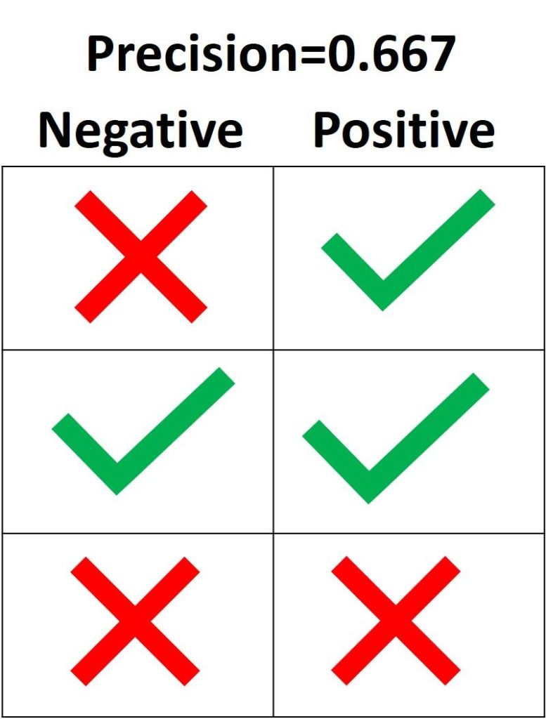
Цель precision – классифицировать все Positive семплы как Positive, не допуская ложных определений Negative как Positive. Согласно следующему рисунку, если все три Positive выборки предсказаны правильно, но один Negative семпл классифицирован неверно, precision составляет 3 / (3 + 1) = 0.75. Таким образом, утверждения модели о том, что выборка относится к классу Positive, корректны с точностью 75%.
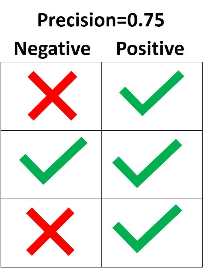
Единственный способ получить 100% precision — это классифицировать все Positive выборки как Positive без классификации Negative как Positive.
В Scikit-learn модуль sklearn.metrics имеет функцию precision_score(), которая получает в качестве аргументов эталонные и предсказанные метки и возвращает precision. Параметр pos_label принимает метку класса Positive (по умолчанию 1).
import sklearn.metrics

y_true = ["positive", "positive", "positive", "negative", "negative", "negative"]
y_pred = ["positive", "positive", "negative", "positive", "negative", "negative"]

precision = sklearn.metrics.precision_score(y_true, y_pred, pos_label="positive")
print(precision)
Вывод: 0.6666666666666666.
Recall
Recall рассчитывается как отношение числа Positive выборок, корректно классифицированных как Positive, к общему количеству Positive семплов. Recall измеряет способность модели обнаруживать выборки, относящиеся к классу Positive. Чем выше recall, тем больше Positive семплов было найдено.
Recall заботится только о том, как классифицируются Positive выборки. Эта метрика не зависит от того, как предсказываются Negative семплы, в отличие от precision. Когда модель верно классифицирует все Positive выборки, recall будет 100%, даже если все представители класса Negative были ошибочно определены как Positive. Давайте посмотрим на несколько примеров.
На следующем изображении представлены 4 разных случая (от A до D), и все они имеют одинаковый recall, равный 0.667. Представленные примеры отличаются только тем, как классифицируются Negative семплы. Например, в случае A все Negative выборки корректно определены, а в случае D – наоборот. Независимо от того, как модель предсказывает класс Negative, recall касается только семплов относящихся к Positive.
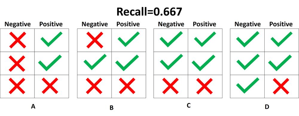
Из 4 случаев, показанных выше, только 2 Positive выборки определены верно. Таким образом, метрика True Positive равна 2. False Negative имеет значение 1, потому что только один Positive семпл классифицируется как Negative. В результате recall будет равен 2 / (2 + 1) = 2/3 = 0.667.
Поскольку не имеет значения, как предсказываются объекты класса Negative, лучше их просто игнорировать, как показано на следующей схеме. При расчете recall необходимо учитывать только Positive выборки.
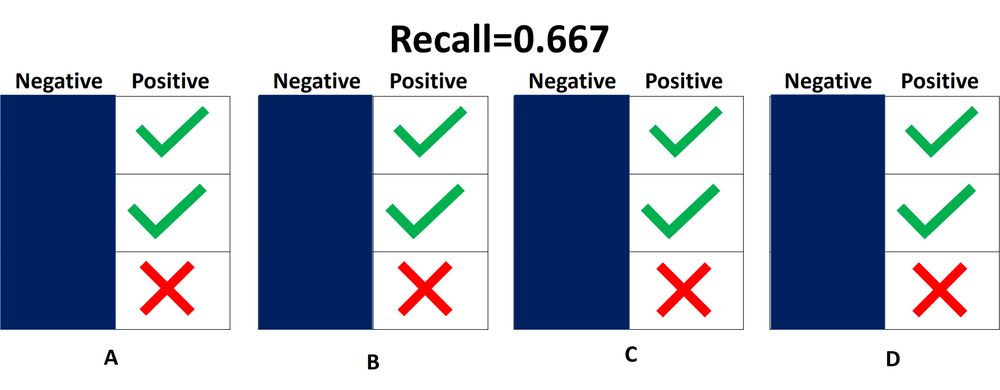
Что означает, когда recall высокий или низкий? Если recall имеет большое значение, все Positive семплы классифицируются верно. Следовательно, модели можно доверять в ее способности обнаруживать представителей класса Positive.
На следующем изображении recall равен 1.0, потому что все Positive семплы были правильно классифицированы. Показатель True Positive равен 3, а False Negative – 0. Таким образом, recall вычисляется как 3 / (3 + 0) = 1. Это означает, что модель обнаружила все Positive выборки. Поскольку recall не учитывает, как предсказываются представители класса Negative, могут присутствовать множество неверно определенных Negative семплов (высокая False Positive метрика).
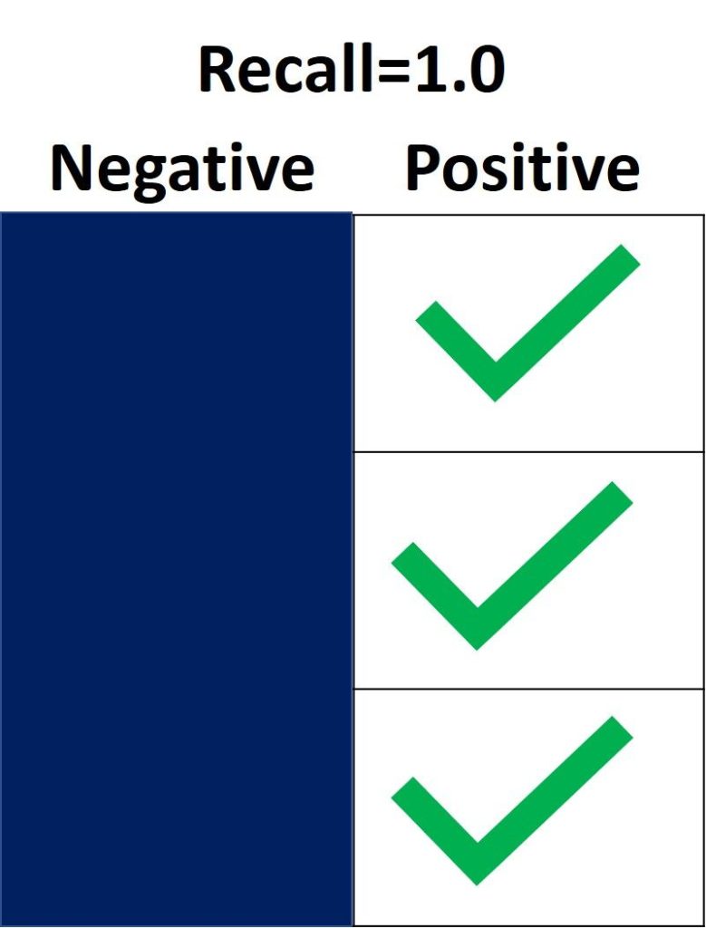
С другой стороны, recall равен 0.0, если не удается обнаружить ни одной Positive выборки. Это означает, что модель обнаружила 0% представителей класса Positive. Показатель True Positive равен 0, а False Negative имеет значение 3. Recall будет равен 0 / (0 + 3) = 0.
Когда recall имеет значение от 0.0 до 1.0, это число отражает процент Positive семплов, которые модель верно классифицировала. Например, если имеется 10 экземпляров Positive и recall равен 0.6, получается, что модель корректно определила 60% объектов класса Positive (т.е. 0.6 * 10 = 6).
Подобно precision_score(), функция repl_score() из модуля sklearn.metrics вычисляет recall. В следующем блоке кода показан пример ее использования.
import sklearn.metrics

y_true = ["positive", "positive", "positive", "negative", "negative", "negative"]
y_pred = ["positive", "positive", "negative", "positive", "negative", "negative"]

recall = sklearn.metrics.recall_score(y_true, y_pred, pos_label="positive")
print(recall)
Вывод: 0.6666666666666666.
После определения precision и recall давайте кратко подведем итоги:
- Precision измеряет надежность модели при классификации Positive семплов, а recall определяет, сколько Positive выборок было корректно предсказано моделью.
- Precision учитывает классификацию как Positive, так и Negative семплов. Recall же использует при расчете только представителей класса Positive. Другими словами, precision зависит как от Negative, так и от Positive-выборок, но recall — только от Positive.
- Precision принимает во внимание, когда семпл определяется как Positive, но не заботится о верной классификации всех объектов класса Positive. Recall в свою очередь учитывает корректность предсказания всех Positive выборок, но не заботится об ошибочной классификации представителей Negative как Positive.
- Когда модель имеет высокий уровень recall метрики, но низкую precision, такая модель правильно определяет большинство Positive семплов, но имеет много ложных срабатываний (классификаций Negative выборок как Positive). Если модель имеет большую precision, но низкий recall, то она делает высокоточные предсказания, определяя класс Positive, но производит всего несколько таких прогнозов.
Некоторые вопросы для проверки понимания:
- Если recall равен 1.0, а в датасете имеются 5 объектов класса Positive, сколько Positive семплов было правильно классифицировано моделью?
- Учитывая, что recall составляет 0.3, когда в наборе данных 30 Positive семплов, сколько представителей класса Positive будет предсказано верно?
- Если recall равен 0.0 и в датасете14 Positive-семплов, сколько корректных предсказаний класса Positive было сделано моделью?
Precision или Recall?
Решение о том, следует ли использовать precision или recall, зависит от типа вашей проблемы. Если цель состоит в том, чтобы обнаружить все positive выборки (не заботясь о том, будут ли negative семплы классифицированы как positive), используйте recall. Используйте precision, если ваша задача связана с комплексным предсказанием класса Positive, то есть учитывая Negative семплы, которые были ошибочно классифицированы как Positive.
Представьте, что вам дали изображение и попросили определить все автомобили внутри него. Какой показатель вы используете? Поскольку цель состоит в том, чтобы обнаружить все автомобили, используйте recall. Такой подход может ошибочно классифицировать некоторые объекты как целевые, но в конечном итоге сработает для предсказания всех автомобилей.
Теперь предположим, что вам дали снимок с результатами маммографии, и вас попросили определить наличие рака. Какой показатель вы используете? Поскольку он обязан быть чувствителен к неверной идентификации изображения как злокачественного, мы должны быть уверены, когда классифицируем снимок как Positive (то есть с раком). Таким образом, предпочтительным показателем в данном случае является precision.
Вывод
В этом руководстве обсуждалась матрица ошибок, вычисление ее 4 метрик (true/false positive/negative) для задач бинарной и мультиклассовой классификации. Используя модуль metrics библиотеки Scikit-learn, мы увидели, как получить матрицу ошибок в Python.
Основываясь на этих 4 показателях, мы перешли к обсуждению accuracy, precision и recall метрик. Каждая из них была определена и использована в нескольких примерах. Модуль sklearn.metrics применяется для расчета каждого вышеперечисленного показателя.
Матрица ошибок – это метрика производительности классифицирующей модели Машинного обучения (ML).
Когда мы получаем данные, то после очистки и предварительной обработки, первым делом передаем их в модель и, конечно же, получаем результат в виде вероятностей. Но как мы можем измерить эффективность нашей модели? Именно здесь матрица ошибок и оказывается в центре внимания.
Матрица ошибок – это показатель успешности классификации, где классов два или более. Это таблица с 4 различными комбинациями сочетаний прогнозируемых и фактических значений.

Давайте рассмотрим значения ячеек (истинно позитивные, ошибочно позитивные, ошибочно негативные, истинно негативные) с помощью «беременной» аналогии.

Истинно позитивное предсказание (True Positive, сокр. TP)
Вы предсказали положительный результат, и женщина действительно беременна.
Истинно отрицательное предсказание (True Negative, TN)
Вы предсказали отрицательный результат, и мужчина действительно не беременен.
Ошибочно положительное предсказание (ошибка типа I, False Positive, FN)
Вы предсказали положительный результат (мужчина беременен), но на самом деле это не так.
Ошибочно отрицательное предсказание (ошибка типа II, False Negative, FN)
Вы предсказали, что женщина не беременна, но на самом деле она беременна.
Давайте разберемся в матрице ошибок с помощью арифметики.
Пример. Мы располагаем датасетом пациентов, у которых диагностируют рак. Зная верный диагноз (столбец целевой переменной «Y на самом деле»), хотим усовершенствовать диагностику с помощью модели Машинного обучения. Модель получила тренировочные данные, и на тестовой части, состоящей из 7 записей (в реальных задачах, конечно, больше) и изображенной ниже, мы оцениваем, насколько хорошо прошло обучение.

Модель сделала свои предсказания для каждого пациента и записала вероятности от 0 до 1 в столбец «Предсказанный Y». Мы округляем эти числа, приводя их к нулю или единице, с помощью порога, равного 0,6 (ниже этого значения – ноль, пациент здоров). Результаты округления попадают в столбец «Предсказанная вероятность»: например, для первой записи модель указала 0,5, что соответствует нулю. В последнем столбце мы анализируем, угадала ли модель.
Теперь, используя простейшие формулы, мы рассчитаем Отзыв (Recall), точность результата измерений (Precision), точность измерений (Accuracy), и наконец поймем разницу между этими метриками.
Отзыв
Из всех положительных значений, которые мы предсказали правильно, сколько на самом деле положительных? Подсчитаем, сколько единиц в столбце «Y на самом деле» (4), это и есть сумма TP + FN. Теперь определим с помощью «Предсказанной вероятности», сколько из них диагностировано верно (2), это и будет TP.
$$Отзыв = frac{TP}{TP + FN} = frac{2}{2 + 2} = frac{1}{2}$$
Точность результата измерений (Precision)
В этом уравнении из неизвестных только FP. Ошибочно диагностированных как больных здесь только одна запись.
$$Точностьspaceрезультатаspaceизмерений = frac{TP}{TP + FP} = frac{2}{2 + 1} = frac{2}{3}$$
Точность измерений (Accuracy)
Последнее значение, которое предстоит экстраполировать из таблицы – TN. Правильно диагностированных моделью здоровых людей здесь 2.
$$Точностьspaceизмерений = frac{TP + TN}{Всегоspaceзначений} = frac{2 + 2}{7} = frac{4}{7}$$
F-мера точности теста
Эти метрики полезны, когда помогают вычислить F-меру – конечный показатель эффективности модели.
$$F-мера = frac{2 * Отзыв * Точностьspaceизмерений}{Отзыв + Точностьspaceизмерений} = frac{2 * frac{1}{2} * frac{2}{3}}{frac{1}{2} + frac{2}{3}} = 0,56$$
Наша скромная модель угадывает лишь 56% процентов диагнозов, и такой результат, как правило, считают промежуточным и работают над улучшением точности модели.
SkLearn
С помощью замечательной библиотеки Scikit-learn мы можем мгновенно определить множество метрик, и матрица ошибок – не исключение.
from sklearn.metrics import confusion_matrix
y_true = [2, 0, 2, 2, 0, 1]
y_pred = [0, 0, 2, 2, 0, 2]
confusion_matrix(y_true, y_pred)
Выводом будет ряд, состоящий из трех списков:
array([[2, 0, 0],
       [0, 0, 1],
       [1, 0, 2]])
Значения диагонали сверху вниз слева направо [2, 0, 2] – это число верно предсказанных значений.
Фото: @opeleye