
- sklearn.metrics.mean_squared_error(y_true, y_pred, *, sample_weight=None, multioutput=‘uniform_average’, squared=True)[source]
-
Mean squared error regression loss.
Read more in the User Guide.
- Parameters:
-
- y_truearray-like of shape (n_samples,) or (n_samples, n_outputs)
-
Ground truth (correct) target values.
- y_predarray-like of shape (n_samples,) or (n_samples, n_outputs)
-
Estimated target values.
- sample_weightarray-like of shape (n_samples,), default=None
-
Sample weights.
- multioutput{‘raw_values’, ‘uniform_average’} or array-like of shape (n_outputs,), default=’uniform_average’
-
Defines aggregating of multiple output values.
Array-like value defines weights used to average errors.- ‘raw_values’ :
-
Returns a full set of errors in case of multioutput input.
- ‘uniform_average’ :
-
Errors of all outputs are averaged with uniform weight.
- squaredbool, default=True
-
If True returns MSE value, if False returns RMSE value.
- Returns:
-
- lossfloat or ndarray of floats
-
A non-negative floating point value (the best value is 0.0), or an
array of floating point values, one for each individual target.
Examples
>>> from sklearn.metrics import mean_squared_error
>>> y_true = [3, -0.5, 2, 7]
>>> y_pred = [2.5, 0.0, 2, 8]
>>> mean_squared_error(y_true, y_pred)
0.375
>>> y_true = [3, -0.5, 2, 7]
>>> y_pred = [2.5, 0.0, 2, 8]
>>> mean_squared_error(y_true, y_pred, squared=False)
0.612...
>>> y_true = [[0.5, 1],[-1, 1],[7, -6]]
>>> y_pred = [[0, 2],[-1, 2],[8, -5]]
>>> mean_squared_error(y_true, y_pred)
0.708...
>>> mean_squared_error(y_true, y_pred, squared=False)
0.822...
>>> mean_squared_error(y_true, y_pred, multioutput='raw_values')
array([0.41666667, 1.        ])
>>> mean_squared_error(y_true, y_pred, multioutput=[0.3, 0.7])
0.825...
Examples using sklearn.metrics.mean_squared_error
Improve Article
Save Article
Like Article
Improve Article
Save Article
Like Article
The Mean Squared Error (MSE) or Mean Squared Deviation (MSD) of an estimator measures the average of error squares i.e. the average squared difference between the estimated values and true value. It is a risk function, corresponding to the expected value of the squared error loss. It is always non – negative and values close to zero are better. The MSE is the second moment of the error (about the origin) and thus incorporates both the variance of the estimator and its bias.
Steps to find the MSE
- Find the equation for the regression line.
(1)

- Insert X values in the equation found in step 1 in order to get the respective Y values i.e.
(2)

- Now subtract the new Y values (i.e. ) from the original Y values. Thus, found values are the error terms. It is also known as the vertical distance of the given point from the regression line.
(3)

- Square the errors found in step 3.
(4)

- Sum up all the squares.
(5)

- Divide the value found in step 5 by the total number of observations.
(6)


Example:
Consider the given data points: (1,1), (2,1), (3,2), (4,2), (5,4)
You can use this online calculator to find the regression equation / line.
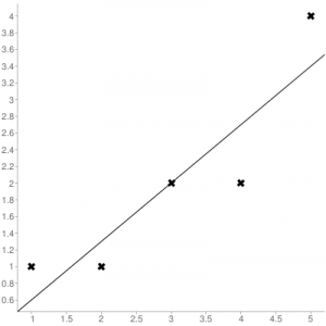
Regression line equation: Y = 0.7X – 0.1
| X | Y |  |
|---|---|---|
| 1 | 1 | 0.6 |
| 2 | 1 | 1.29 |
| 3 | 2 | 1.99 |
| 4 | 2 | 2.69 |
| 5 | 4 | 3.4 |
Now, using formula found for MSE in step 6 above, we can get MSE = 0.21606
MSE using scikit – learn:
from sklearn.metrics import mean_squared_error
Y_true = [1,1,2,2,4]
Y_pred = [0.6,1.29,1.99,2.69,3.4]
mean_squared_error(Y_true,Y_pred)
Output: 0.21606
MSE using Numpy module:
import numpy as np
Y_true = [1,1,2,2,4]
Y_pred = [0.6,1.29,1.99,2.69,3.4]
MSE = np.square(np.subtract(Y_true,Y_pred)).mean()
Output: 0.21606
Last Updated :
30 Jun, 2019
Like Article
Save Article
Время на прочтение
4 мин
Количество просмотров 3.7K

Функции потерь Python являются важной частью моделей машинного обучения. Эти функции показывают, насколько сильно предсказанный моделью результат отличается от фактического.
Существует несколько способов вычислить эту разницу. В этом материале мы рассмотрим некоторые из наиболее распространенных функций потерь.
Ниже будут рассмотрены следующие четыре функции потерь.
-
Среднеквадратическая ошибка
-
Среднеквадратическая ошибка
-
Средняя абсолютная ошибка
-
Кросс-энтропийные потери
Из этих четырех функций потерь первые три применяются к модели классификации.
1. Среднеквадратическая ошибка (MSE)
Среднеквадратичная ошибка (MSE) рассчитывается как среднее значение квадратов разностей между прогнозируемыми и фактически наблюдаемыми значениями. Математически это можно выразить следующим образом:
Реализация MSE на языке Python выглядит следующим образом:
import numpy as np # импортируем библиотеку numpy
def mean_squared_error(act, pred): # функция

   diff = pred - act # находим разницу между прогнозируемыми и наблюдаемыми значениями
   differences_squared = diff ** 2 # возводим в квадрат (чтобы избавиться от отрицательных значений)
   mean_diff = differences_squared.mean() # находим среднее значение

   return mean_diff

act = np.array([1.1,2,1.7]) # создаем список актуальных значений
pred = np.array([1,1.7,1.5]) # список прогнозируемых значений

print(mean_squared_error(act,pred))
Выход :
0.04666666666666667Вы также можете использовать mean_squared_error из sklearn для расчета MSE. Вот как работает функция:
from sklearn.metrics import mean_squared_error
act = np.array([1.1,2,1.7])
pred = np.array([1,1.7,1.5])
mean_squared_error(act, pred)
Выход :
0.04666666666666667
2. Корень среднеквадратической ошибки (RMSE)
Итак, ранее, для того, чтобы найти действительную ошибку среди между прогнозируемыми и фактически наблюдаемыми значениями (там могли быть положительные и отрицательные значения), мы возводили их в квадрат (для того чтобы отрицательные значения участвовали в расчетах в полной мере). Это была среднеквадратичная ошибка (MSE).
Корень среднеквадратической ошибки (RMSE) мы используем для того чтобы избавиться от квадратной степени, в которую мы ранее возвели действительную ошибку среди между прогнозируемыми и фактически наблюдаемыми значениями. Математически мы можем представить это следующим образом:
Реализация Python для RMSE выглядит следующим образом:
import numpy as np
def root_mean_squared_error(act, pred):

   diff = pred - act # находим разницу между прогнозируемыми и наблюдаемыми значениями
   differences_squared = diff ** 2 # возводим в квадрат
   mean_diff = differences_squared.mean() # находим среднее значение
   rmse_val = np.sqrt(mean_diff) # извлекаем квадратный корень
   return rmse_val

act = np.array([1.1,2,1.7])
pred = np.array([1,1.7,1.5])

print(root_mean_squared_error(act,pred))
Выход :
0.21602468994692867
Вы также можете использовать mean_squared_error из sklearn для расчета RMSE. Давайте посмотрим, как реализовать RMSE, используя ту же функцию:
from sklearn.metrics import mean_squared_error
act = np.array([1.1,2,1.7])
pred = np.array([1,1.7,1.5])
mean_squared_error(act, pred, squared = False) #Если установлено значение False, функция возвращает значение RMSE.
Выход :
0.21602468994692867
Если для параметра squared установлено значение True, функция возвращает значение MSE. Если установлено значение False, функция возвращает значение RMSE.
3. Средняя абсолютная ошибка (MAE)
Средняя абсолютная ошибка (MAE) рассчитывается как среднее значение абсолютной разницы между прогнозами и фактическими наблюдениями. Математически мы можем представить это следующим образом:
Реализация Python для MAE выглядит следующим образом:
import numpy as np
def mean_absolute_error(act, pred): #
    diff = pred - act # находим разницу между прогнозируемыми и наблюдаемыми значениями
    abs_diff = np.absolute(diff) # находим абсолютную разность между прогнозами и фактическими наблюдениями.
    mean_diff = abs_diff.mean() # находим среднее значение
    return mean_diff

act = np.array([1.1,2,1.7])
pred = np.array([1,1.7,1.5])
mean_absolute_error(act,pred)
Выход :
0.20000000000000004
Вы также можете использовать mean_absolute_error из sklearn для расчета MAE.
from sklearn.metrics import mean_absolute_error
act = np.array([1.1,2,1.7])
pred = np.array([1,1.7,1.5])
mean_absolute_error(act, pred)
Выход :
0.20000000000000004
4. Функция потерь перекрестной энтропии в Python
Функция потерь перекрестной энтропии также известна как отрицательная логарифмическая вероятность. Это чаще всего используется для задач классификации. Проблема классификации — это проблема, в которой вы классифицируете пример как принадлежащий к одному из более чем двух классов.
Давайте посмотрим, как вычислить ошибку в случае проблемы бинарной классификации.
Давайте рассмотрим проблему классификации, когда модель пытается провести классификацию между собакой и кошкой.
Код Python для поиска ошибки приведен ниже.
from sklearn.metrics import log_loss
log_loss(["Dog", "Cat", "Cat", "Dog"],[[.1, .9], [.9, .1], [.8, .2], [.35, .65]])
Выход :
0.21616187468057912
Мы используем метод log_loss из sklearn.
Первый аргумент в вызове функции — это список правильных меток классов для каждого входа. Второй аргумент — это список вероятностей, предсказанных моделью.
Вероятности представлены в следующем формате:
[P(dog), P(cat)]
Заключение
Это руководство было посвящено функциям потерь в Python. Мы рассмотрели различные функции потерь как для задач регрессии, так и для задач классификации. Надеюсь, вам понравился материал, ведь все было достаточно легко и понятно!
Кстати, для тех, кто хотел бы пойти дальше в изучении функций потерь, мы предлагаем разобрать одну вот такую — это очень интересная функция потерь Triplet Loss в Python (функцию тройных потерь), которую для вас любезно подготовил автор.
The mean squared error is a common way to measure the prediction accuracy of a model. In this tutorial, you’ll learn how to calculate the mean squared error in Python. You’ll start off by learning what the mean squared error represents. Then you’ll learn how to do this using Scikit-Learn (sklean), Numpy, as well as from scratch.
What is the Mean Squared Error
The mean squared error measures the average of the squares of the errors. What this means, is that it returns the average of the sums of the square of each difference between the estimated value and the true value.
The MSE is always positive, though it can be 0 if the predictions are completely accurate. It incorporates the variance of the estimator (how widely spread the estimates are) and its bias (how different the estimated values are from their true values).
The formula looks like below:

Now that you have an understanding of how to calculate the MSE, let’s take a look at how it can be calculated using Python.
Interpreting the Mean Squared Error
The mean squared error is always 0 or positive. When a MSE is larger, this is an indication that the linear regression model doesn’t accurately predict the model.
An important piece to note is that the MSE is sensitive to outliers. This is because it calculates the average of every data point’s error. Because of this, a larger error on outliers will amplify the MSE.
There is no “target” value for the MSE. The MSE can, however, be a good indicator of how well a model fits your data. It can also give you an indicator of choosing one model over another.
Loading a Sample Pandas DataFrame
Let’s start off by loading a sample Pandas DataFrame. If you want to follow along with this tutorial line-by-line, simply copy the code below and paste it into your favorite code editor.
# Importing a sample Pandas DataFrame
import pandas as pd

df = pd.DataFrame.from_dict({
    'x': [1,2,3,4,5,6,7,8,9,10],
    'y': [1,2,2,4,4,5,6,7,9,10]})

print(df.head())
#    x  y
# 0  1  1
# 1  2  2
# 2  3  2
# 3  4  4
# 4  5  4
You can see that the editor has loaded a DataFrame containing values for variables x and y. We can plot this data out, including the line of best fit using Seaborn’s .regplot() function:
# Plotting a line of best fit
import seaborn as sns
import matplotlib.pyplot as plt
sns.regplot(data=df, x='x', y='y', ci=None)
plt.ylim(bottom=0)
plt.xlim(left=0)
plt.show()
This returns the following visualization:
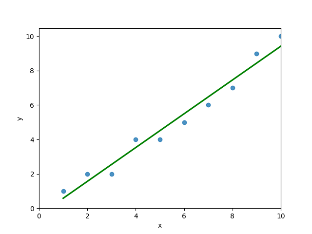
The mean squared error calculates the average of the sum of the squared differences between a data point and the line of best fit. By virtue of this, the lower a mean sqared error, the more better the line represents the relationship.
We can calculate this line of best using Scikit-Learn. You can learn about this in this in-depth tutorial on linear regression in sklearn. The code below predicts values for each x value using the linear model:
# Calculating prediction y values in sklearn
from sklearn.linear_model import LinearRegression

model = LinearRegression()
model.fit(df[['x']], df['y'])
y_2 = model.predict(df[['x']])
df['y_predicted'] = y_2
print(df.head())

# Returns:
#    x  y  y_predicted
# 0  1  1     0.581818
# 1  2  2     1.563636
# 2  3  2     2.545455
# 3  4  4     3.527273
# 4  5  4     4.509091
Calculating the Mean Squared Error with Scikit-Learn
The simplest way to calculate a mean squared error is to use Scikit-Learn (sklearn). The metrics module comes with a function, mean_squared_error() which allows you to pass in true and predicted values.
Let’s see how to calculate the MSE with sklearn:
# Calculating the MSE with sklearn
from sklearn.metrics import mean_squared_error
mse = mean_squared_error(df['y'], df['y_predicted'])
print(mse)

# Returns: 0.24727272727272714
This approach works very well when you’re already importing Scikit-Learn. That said, the function works easily on a Pandas DataFrame, as shown above.
In the next section, you’ll learn how to calculate the MSE with Numpy using a custom function.
Calculating the Mean Squared Error from Scratch using Numpy
Numpy itself doesn’t come with a function to calculate the mean squared error, but you can easily define a custom function to do this. We can make use of the subtract() function to subtract arrays element-wise.
# Definiting a custom function to calculate the MSE
import numpy as np

def mse(actual, predicted):
    actual = np.array(actual)
    predicted = np.array(predicted)
    differences = np.subtract(actual, predicted)
    squared_differences = np.square(differences)
    return squared_differences.mean()

print(mse(df['y'], df['y_predicted']))

# Returns: 0.24727272727272714
The code above is a bit verbose, but it shows how the function operates. We can cut down the code significantly, as shown below:
# A shorter version of the code above
import numpy as np

def mse(actual, predicted):
    return np.square(np.subtract(np.array(actual), np.array(predicted))).mean()

print(mse(df['y'], df['y_predicted']))

# Returns: 0.24727272727272714
Conclusion
In this tutorial, you learned what the mean squared error is and how it can be calculated using Python. First, you learned how to use Scikit-Learn’s mean_squared_error() function and then you built a custom function using Numpy.
The MSE is an important metric to use in evaluating the performance of your machine learning models. While Scikit-Learn abstracts the way in which the metric is calculated, understanding how it can be implemented from scratch can be a helpful tool.
Additional Resources
To learn more about related topics, check out the tutorials below:
- Pandas Variance: Calculating Variance of a Pandas Dataframe Column
- Calculate the Pearson Correlation Coefficient in Python
- How to Calculate a Z-Score in Python (4 Ways)
- Official Documentation from Scikit-Learn
17 авг. 2022 г.
читать 1 мин
Среднеквадратическая ошибка (MSE) — это распространенный способ измерения точности предсказания модели. Он рассчитывается как:
MSE = (1/n) * Σ(фактическое – прогноз) 2
куда:
- Σ — причудливый символ, означающий «сумма».
- n – размер выборки
- фактический – фактическое значение данных
- прогноз – прогнозируемое значение данных
Чем ниже значение MSE, тем лучше модель способна точно предсказывать значения.
Как рассчитать MSE в Python
Мы можем создать простую функцию для вычисления MSE в Python:
import numpy as np

def mse(actual, pred):
 actual, pred = np.array(actual), np.array(pred)
 return np.square(np.subtract(actual,pred)).mean()
Затем мы можем использовать эту функцию для вычисления MSE для двух массивов: одного, содержащего фактические значения данных, и другого, содержащего прогнозируемые значения данных.
actual = [12, 13, 14, 15, 15, 22, 27]
pred = [11, 13, 14, 14, 15, 16, 18]

mse(actual, pred)

17.0
Среднеквадратическая ошибка (MSE) для этой модели оказывается равной 17,0 .
На практике среднеквадратическая ошибка (RMSE) чаще используется для оценки точности модели. Как следует из названия, это просто квадратный корень из среднеквадратичной ошибки.
Мы можем определить аналогичную функцию для вычисления RMSE:
import numpy as np

def rmse(actual, pred):
 actual, pred = np.array(actual), np.array(pred)
 return np.sqrt(np.square(np.subtract(actual,pred)).mean())
Затем мы можем использовать эту функцию для вычисления RMSE для двух массивов: одного, содержащего фактические значения данных, и другого, содержащего прогнозируемые значения данных.
actual = [12, 13, 14, 15, 15, 22, 27]
pred = [11, 13, 14, 14, 15, 16, 18]

rmse(actual, pred)

4.1231
Среднеквадратическая ошибка (RMSE) для этой модели оказывается равной 4,1231 .
Дополнительные ресурсы
Калькулятор среднеквадратичной ошибки (MSE)
Как рассчитать среднеквадратичную ошибку (MSE) в Excel

Функции потерь Python являются важной частью моделей машинного обучения. Эти функции показывают, насколько сильно предсказанный моделью результат отличается от фактического.
Существует несколько способов вычислить эту разницу. В этом материале мы рассмотрим некоторые из наиболее распространенных функций потерь.
В этом уроке будут рассмотрены следующие четыре функции потерь.
- Среднеквадратическая ошибка
- Среднеквадратическая ошибка
- Средняя абсолютная ошибка
- Кросс-энтропийные потери
Из этих четырех функций потерь первые три применяются к модели классификации.
Реализация функций потерь в Python
1. Среднеквадратическая ошибка (MSE)
Среднеквадратичная ошибка (MSE) рассчитывается как среднее значение квадратов разностей между прогнозируемыми и фактически наблюдаемыми значениями. Математически это можно выразить следующим образом:
Реализация MSE на языке Python выглядит следующим образом:
import numpy as np
def mean_squared_error(act, pred):

   diff = pred - act
   differences_squared = diff ** 2
   mean_diff = differences_squared.mean()

   return mean_diff

act = np.array([1.1,2,1.7])
pred = np.array([1,1.7,1.5])

print(mean_squared_error(act,pred))
Выход :
Вы также можете использовать mean_squared_error из sklearn для расчета MSE. Вот как работает функция:
from sklearn.metrics import mean_squared_error
act = np.array([1.1,2,1.7])
pred = np.array([1,1.7,1.5])
mean_squared_error(act, pred)
Выход :
2. Среднеквадратическая ошибка (RMSE)
Стандартное отклонение (RMSD) или среднеквадратичная ошибка (RMSE) — это часто используемая мера разницы между значением (выборочным или общим), предсказанным моделью или оценщиком, и наблюдаемым значением. и наблюдаемыми значениями, или квадратный корень из разницы между ними по второму моменту выборки, или среднеквадратичное значение этих разниц. Эти отклонения называются остатками при расчете по выборке данных, используемых для оценки, и ошибками (или ошибками предсказания) при расчете вне выборки. RMSD используется как единая мера предсказательной силы, включающая величину ошибки предсказания в разных точках данных. RMSD зависит от масштаба и поэтому сравнивает точность ошибок предсказания различных моделей для данного набора данных, а не между наборами данных.
RMSD всегда неотрицателен, при этом значение нуля (что редко достигается на практике) указывает на идеальное согласие с данными. В целом, низкий RMSD лучше, чем высокий RMSD. Однако эта мера зависит от используемой числовой шкалы, что делает невозможным сравнение между различными типами данных.
RMSD — это квадратный корень из среднего квадрата ошибок. Влияние каждой ошибки на RMSD пропорционально размеру квадрата ошибки, поэтому большие ошибки оказывают непропорционально большое влияние на RMSD. Поэтому RMSD чувствителен к выбросам.
Среднеквадратическая ошибка (RMSE) рассчитывается как квадратный корень из среднеквадратичной ошибки. Математически мы можем представить это следующим образом:
Реализация Python для RMSE выглядит следующим образом:
import numpy as np
def root_mean_squared_error(act, pred):

   diff = pred - act
   differences_squared = diff ** 2
   mean_diff = differences_squared.mean()
   rmse_val = np.sqrt(mean_diff)
   return rmse_val

act = np.array([1.1,2,1.7])
pred = np.array([1,1.7,1.5])

print(root_mean_squared_error(act,pred))
Выход :
Вы также можете использовать mean_squared_error из sklearn для расчета RMSE. Давайте посмотрим, как реализовать RMSE, используя ту же функцию:
from sklearn.metrics import mean_squared_error
act = np.array([1.1,2,1.7])
pred = np.array([1,1.7,1.5])
mean_squared_error(act, pred, squared = False) #Если установлено значение False, функция возвращает значение RMSE.
Выход :
Если для параметра squared установлено значение True, функция возвращает значение MSE. Если установлено значение False, функция возвращает значение RMSE.
3. Средняя абсолютная ошибка (MAE)
Средняя абсолютная ошибка (MAE) рассчитывается как среднее значение абсолютной разницы между прогнозами и фактическими наблюдениями. Математически мы можем представить это следующим образом:
Реализация Python для MAE выглядит следующим образом:
import numpy as np
def mean_absolute_error(act, pred):
    diff = pred - act
    abs_diff = np.absolute(diff)
    mean_diff = abs_diff.mean()
    return mean_diff

act = np.array([1.1,2,1.7])
pred = np.array([1,1.7,1.5])
mean_absolute_error(act,pred)
Выход :
Вы также можете использовать mean_absolute_error из sklearn для расчета MAE.
from sklearn.metrics import mean_absolute_error
act = np.array([1.1,2,1.7])
pred = np.array([1,1.7,1.5])
mean_absolute_error(act, pred)
Выход :
4. Функция кросс-энтропийной потери в Python
Перекрестная энтропийная потеря также известна как отрицательная логарифмическая вероятность. Это чаще всего используется для задач классификации. Проблема классификации — это проблема, в которой вы классифицируете пример как принадлежащий к одному из более чем двух классов.
Давайте посмотрим, как вычислить ошибку в случае проблемы бинарной классификации.
Давайте рассмотрим проблему классификации, когда модель пытается провести классификацию между собакой и кошкой.
Код Python для поиска ошибки приведен ниже.
from sklearn.metrics import log_loss
log_loss(["Dog", "Cat", "Cat", "Dog"],[[.1, .9], [.9, .1], [.8, .2], [.35, .65]])
Выход :
Мы используем метод log_loss из sklearn.
Первый аргумент в вызове функции — это список правильных меток классов для каждого входа. Второй аргумент — это список вероятностей, предсказанных моделью.
Вероятности представлены в следующем формате:
Заключение
Это руководство было посвящено функциям потерь в Python. Мы рассмотрели различные функции потерь как для задач регрессии, так и для задач классификации. Надеюсь, вам было весело учиться вместе с нами!
What is RMSE? Also known as MSE, RMD, or RMS. What problem does it solve?
If you understand RMSE: (Root mean squared error), MSE: (Mean Squared Error) RMD (Root mean squared deviation) and RMS: (Root Mean Squared), then asking for a library to calculate this for you is unnecessary over-engineering. All these can be intuitively written in a single line of code. rmse, mse, rmd, and rms are different names for the same thing.
RMSE answers: «How similar, on average, are the numbers in list1 to list2?». The two lists must be the same size. Wash out the noise between any two given elements, wash out the size of the data collected, and get a single number result».
Intuition and ELI5 for RMSE. What problem does it solve?:
Imagine you are learning to throw darts at a dart board. Every day you practice for one hour. You want to figure out if you are getting better or getting worse. So every day you make 10 throws and measure the distance between the bullseye and where your dart hit.
You make a list of those numbers list1. Use the root mean squared error between the distances at day 1 and a list2 containing all zeros. Do the same on the 2nd and nth days. What you will get is a single number that hopefully decreases over time. When your RMSE number is zero, you hit bullseyes every time. If the rmse number goes up, you are getting worse.
Example in calculating root mean squared error in python:
import numpy as np
d = [0.000, 0.166, 0.333]   #ideal target distances, these can be all zeros.
p = [0.000, 0.254, 0.998]   #your performance goes here

print("d is: " + str(["%.8f" % elem for elem in d]))
print("p is: " + str(["%.8f" % elem for elem in p]))

def rmse(predictions, targets):
    return np.sqrt(((predictions - targets) ** 2).mean())

rmse_val = rmse(np.array(d), np.array(p))
print("rms error is: " + str(rmse_val))
Which prints:
d is: ['0.00000000', '0.16600000', '0.33300000']
p is: ['0.00000000', '0.25400000', '0.99800000']
rms error between lists d and p is: 0.387284994115
The mathematical notation:

Glyph Legend: n is a whole positive integer representing the number of throws. i represents a whole positive integer counter that enumerates sum. d stands for the ideal distances, the list2 containing all zeros in above example. p stands for performance, the list1 in the above example. superscript 2 stands for numeric squared. di is the i’th index of d. pi is the i’th index of p.
The rmse done in small steps so it can be understood:
def rmse(predictions, targets):

    differences = predictions - targets                       #the DIFFERENCEs.

    differences_squared = differences ** 2                    #the SQUAREs of ^

    mean_of_differences_squared = differences_squared.mean()  #the MEAN of ^

    rmse_val = np.sqrt(mean_of_differences_squared)           #ROOT of ^

    return rmse_val                                           #get the ^
How does every step of RMSE work:
Subtracting one number from another gives you the distance between them.
8 - 5 = 3         #absolute distance between 8 and 5 is +3
-20 - 10 = -30    #absolute distance between -20 and 10 is +30
If you multiply any number times itself, the result is always positive because negative times negative is positive:
3*3     = 9   = positive
-30*-30 = 900 = positive
Add them all up, but wait, then an array with many elements would have a larger error than a small array, so average them by the number of elements.
But we squared them all earlier, to force them positive. Undo that damage with a square root.
That leaves you with a single number that represents, on average, the distance between every value of list1 to it’s corresponding element value of list2.
If the RMSE value goes down over time we are happy because variance is decreasing. «Shrinking the Variance» here is a primitive kind of machine learning algorithm.
RMSE isn’t the most accurate line fitting strategy, total least squares is:
Root mean squared error measures the vertical distance between the point and the line, so if your data is shaped like a banana, flat near the bottom and steep near the top, then the RMSE will report greater distances to points high, but short distances to points low when in fact the distances are equivalent. This causes a skew where the line prefers to be closer to points high than low.
If this is a problem the total least squares method fixes this:
https://mubaris.com/posts/linear-regression
Gotchas that can break this RMSE function:
If there are nulls or infinity in either input list, then output rmse value is is going to not make sense. There are three strategies to deal with nulls / missing values / infinities in either list: Ignore that component, zero it out or add a best guess or a uniform random noise to all timesteps. Each remedy has its pros and cons depending on what your data means. In general ignoring any component with a missing value is preferred, but this biases the RMSE toward zero making you think performance has improved when it really hasn’t. Adding random noise on a best guess could be preferred if there are lots of missing values.
In order to guarantee relative correctness of the RMSE output, you must eliminate all nulls/infinites from the input.
RMSE has zero tolerance for outlier data points which don’t belong
Root mean squared error squares relies on all data being right and all are counted as equal. That means one stray point that’s way out in left field is going to totally ruin the whole calculation. To handle outlier data points and dismiss their tremendous influence after a certain threshold, see Robust estimators that build in a threshold for dismissal of outliers as extreme rare events that don’t need their outlandish results to change our behavior.
In this article, we are going to learn how to calculate the mean squared error in python? We are using two python libraries to calculate the mean squared error. NumPy and sklearn are the libraries we are going to use here. Also, we will learn how to calculate without using any module.
MSE is also useful for regression problems that are normally distributed. It is the mean squared error. So the squared error between the predicted values and the actual values. The summation of all the data points of the square difference between the predicted and actual values is divided by the no. of data points.
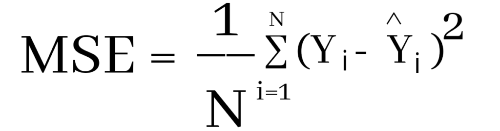
Where Yi and Ŷi represent the actual values and the predicted values, the difference between them is squared.
Derivation of Mean Squared Error
First to find the regression line for the values (1,3), (2,2), (3,6), (4,1), (5,5). The regression value for the value is y=1.6+0.4x. Next to find the new Y values. The new values for y are tabulated below.
| Given x value | Calculating y value | New y value |
|---|---|---|
| 1 | 1.6+0.4(1) | 2 |
| 2 | 1.6+0.4(2) | 2.4 |
| 3 | 1.6+0.4(3) | 2.8 |
| 4 | 1.6+0.4(4) | 3.2 |
| 5 | 1.6+0.4(5) | 3.6 |
Now to find the error ( Yi – Ŷi )
We have to square all the errors
By adding all the errors we will get the MSE
Line regression graph
Let us consider the values (1,3), (2,2), (3,6), (4,1), (5,5) to plot the graph.
The straight line represents the predicted value in this graph, and the points represent the actual data. The difference between this line and the points is squared, known as mean squared error.
Also, Read | How to Calculate Square Root in Python
To get the Mean Squared Error in Python using NumPy
import numpy as np
true_value_of_y= [3,2,6,1,5]
predicted_value_of_y= [2.0,2.4,2.8,3.2,3.6]
MSE = np.square(np.subtract(true_value_of_y,predicted_value_of_y)).mean()
print(MSE)
Importing numpy library as np. Creating two variables. true_value_of_y holds an original value. predicted_value_of_y holds a calculated value. Next, giving the formula to calculate the mean squared error.
Output
3.6400000000000006
To get the MSE using sklearn
sklearn is a library that is used for many mathematical calculations in python. Here we are going to use this library to calculate the MSE
Syntax
sklearn.metrices.mean_squared_error(y_true, y_pred, *, sample_weight=None, multioutput='uniform_average', squared=True)
Parameters
- y_true – true value of y
- y_pred – predicted value of y
- sample_weight
- multioutput
- raw_values
- uniform_average
- squared
Returns
Mean squared error.
Code
from sklearn.metrics import mean_squared_error
true_value_of_y= [3,2,6,1,5]
predicted_value_of_y= [2.0,2.4,2.8,3.2,3.6]
mean_squared_error(true_value_of_y,predicted_value_of_y)
print(mean_squared_error(true_value_of_y,predicted_value_of_y))
From sklearn.metrices library importing mean_squared_error. Creating two variables. true_value_of_y holds an original value. predicted_value_of_y holds a calculated value. Next, giving the formula to calculate the mean squared error.
Output
3.6400000000000006
Calculating Mean Squared Error Without Using any Modules
true_value_of_y = [3,2,6,1,5]
predicted_value_of_y = [2.0,2.4,2.8,3.2,3.6]
summation_of_value = 0
n = len(true_value_of_y)
for i in range (0,n):
  difference_of_value = true_value_of_y[i] - predicted_value_of_y[i]
  squared_difference = difference_of_value**2
  summation_of_value = summation_of_value + squared_difference
MSE = summation_of_value/n
print ("The Mean Squared Error is: " , MSE)
Declaring the true values and the predicted values to two different variables. Initializing the variable summation_of_value is zero to store the values. len() function is useful to check the number of values in true_value_of_y. Creating for loop to iterate. Calculating the difference between true_value and the predicted_value. Next getting the square of the difference. Adding all the squared differences, we will get the MSE.
Output
The Mean Squared Error is: 3.6400000000000006
Calculate Mean Squared Error Using Negative Values
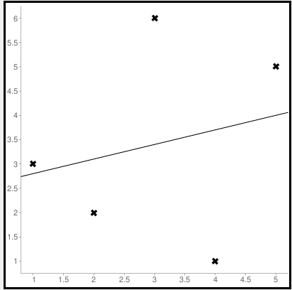
Now let us consider some negative values to calculate MSE. The values are (1,2), (3,-1), (5,0.6), (4,-0.7), (2,-0.2). The regression line equation is y=1.13-0.33x
The line regression graph for this value is:
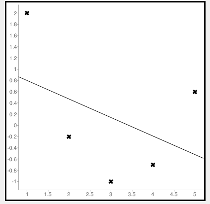
New y values for this will be:
| Given x value | Calculating y value | New y value |
|---|---|---|
| 1 | 1.13-033(1) | 0.9 |
| 3 | 1.13-033(3) | 0.1 |
| 5 | 1.13-033(5) | -0.4 |
| 4 | 1.13-033(4) | -0.1 |
| 2 | 1.13-033(2) | 0.6 |
Code
>>> from sklearn.metrics import mean_squared_error
>>> y_true = [2,-1,0.6,-0.7,-0.2]
>>> y_pred = [0.9,0.1,-0.4,-0.1,0.6]
>>> mean_squared_error(y_true, y_pred)
First, importing a module. Declaring values to the variables. Here we are using negative value to calculate. Using the mean_squared_error module, we are calculating the MSE.
Output
0.884
Bonus: Gradient Descent
Gradient Descent is used to find the local minimum of the functions. In this case, the functions need to be differentiable. The basic idea is to move in the direction opposite from the derivate at any point.
The following code works on a set of values that are available on the Github repository.
Code:
#!/usr/bin/python
# -*- coding: utf-8 -*-
from numpy import *


def compute_error(b, m, points):
    totalError = 0
    for i in range(0, len(points)):
        x = points[i, 0]
        y = points[i, 1]
        totalError += (y - (m * x + b)) ** 2
    return totalError / float(len(points))


def gradient_step(
    b_current,
    m_current,
    points,
    learningRate,
    ):
    b_gradient = 0
    m_gradient = 0
    N = float(len(points))
    for i in range(0, len(points)):
        x = points[i, 0]
        y = points[i, 1]
        b_gradient += -(2 / N) * (y - (m_current * x + b_current))
        m_gradient += -(2 / N) * x * (y - (m_current * x + b_current))
    new_b = b_current - learningRate * b_gradient
    new_m = m_current - learningRate * m_gradient
    return [new_b, new_m]


def gradient_descent_runner(
    points,
    starting_b,
    starting_m,
    learning_rate,
    iterations,
    ):
    b = starting_b
    m = starting_m
    for i in range(iterations):
        (b, m) = gradient_step(b, m, array(points), learning_rate)
    return [b, m]


def main():
    points = genfromtxt('data.csv', delimiter=',')
    learning_rate = 0.00001
    initial_b = 0
    initial_m = 0
    iterations = 10000
    print('Starting gradient descent at b = {0}, m = {1}, error = {2}'.format(initial_b,
            initial_m, compute_error(initial_b, initial_m, points)))
    print('Running...')
    [b, m] = gradient_descent_runner(points, initial_b, initial_m,
            learning_rate, iterations)
    print('After {0} iterations b = {1}, m = {2}, error = {3}'.format(iterations,
            b, m, compute_error(b, m, points)))


if __name__ == '__main__':
    main()
Output:
Starting gradient descent at b = 0, m = 0, error = 5671.844671124282
Running...
After 10000 iterations b = 0.11558415090685024, m = 1.3769012288001614, error = 212.26220312358794
1. What is the pip command to install numpy?
pip install numpy
2. What is the pip command to install sklearn.metrices library?
pip install sklearn
3. What is the expansion of MSE?
The expansion of MSE is Mean Squared Error.
Conclusion
In this article, we have learned about the mean squared error. It is effortless to calculate. This is useful for loss function for least squares regression. The formula for the MSE is easy to memorize. We hope this article is handy and easy to understand.
Computes the mean of squares of errors between labels and predictions.
Inherits From: Loss
View aliases
Main aliases
tf.losses.MeanSquaredError
Compat aliases for migration
See
Migration guide for
more details.
tf.compat.v1.keras.losses.MeanSquaredError
tf.keras.losses.MeanSquaredError(
    reduction=losses_utils.ReductionV2.AUTO,
    name='mean_squared_error'
)
Used in the notebooks
| Used in the guide | Used in the tutorials |
|---|---|
|
|
loss = square(y_true - y_pred)
Standalone usage:
y_true = [[0., 1.], [0., 0.]]y_pred = [[1., 1.], [1., 0.]]# Using 'auto'/'sum_over_batch_size' reduction type.mse = tf.keras.losses.MeanSquaredError()mse(y_true, y_pred).numpy()0.5
# Calling with 'sample_weight'.mse(y_true, y_pred, sample_weight=[0.7, 0.3]).numpy()0.25
# Using 'sum' reduction type.mse = tf.keras.losses.MeanSquaredError(reduction=tf.keras.losses.Reduction.SUM)mse(y_true, y_pred).numpy()1.0
# Using 'none' reduction type.mse = tf.keras.losses.MeanSquaredError(reduction=tf.keras.losses.Reduction.NONE)mse(y_true, y_pred).numpy()array([0.5, 0.5], dtype=float32)
Usage with the compile() API:
model.compile(optimizer='sgd', loss=tf.keras.losses.MeanSquaredError())
Args |
|
|---|---|
reduction
|
Type of tf.keras.losses.Reduction to apply toloss. Default value is AUTO. AUTO indicates that the reductionoption will be determined by the usage context. For almost all cases this defaults to SUM_OVER_BATCH_SIZE. When used under atf.distribute.Strategy, except via Model.compile() andModel.fit(), using AUTO or SUM_OVER_BATCH_SIZEwill raise an error. Please see this custom training tutorial for more details. |
name
|
Optional name for the instance. Defaults to ‘mean_squared_error’. |
Methods
from_config
View source
@classmethodfrom_config( config )
Instantiates a Loss from its config (output of get_config()).
| Args | |
|---|---|
config
|
Output of get_config().
|
| Returns |
|---|
A keras.losses.Loss instance.
|
get_config
View source
get_config()
Returns the config dictionary for a Loss instance.
__call__
View source
__call__(
    y_true, y_pred, sample_weight=None
)
Invokes the Loss instance.
| Args | |
|---|---|
y_true
|
Ground truth values. shape = [batch_size, d0, .. dN], exceptsparse loss functions such as sparse categorical crossentropy where shape = [batch_size, d0, .. dN-1]
|
y_pred
|
The predicted values. shape = [batch_size, d0, .. dN]
|
sample_weight
|
Optional sample_weight acts as a coefficient for theloss. If a scalar is provided, then the loss is simply scaled by the given value. If sample_weight is a tensor of size [batch_size],then the total loss for each sample of the batch is rescaled by the corresponding element in the sample_weight vector. If the shape ofsample_weight is [batch_size, d0, .. dN-1] (or can bebroadcasted to this shape), then each loss element of y_pred isscaled by the corresponding value of sample_weight. (Noteon dN-1: all loss functions reduce by 1 dimension, usuallyaxis=-1.) |
| Returns |
|---|
Weighted loss float Tensor. If reduction is NONE, this hasshape [batch_size, d0, .. dN-1]; otherwise, it is scalar. (NotedN-1 because all loss functions reduce by 1 dimension, usuallyaxis=-1.) |
| Raises | |
|---|---|
ValueError
|
If the shape of sample_weight is invalid.
|