Среднеквадратичная ошибка сигнала - Не ошибается лишь тот, кто ничего не делает!

Замена нелинейного
звена линеаризованной моделью позволяет
использовать принцип суперпозиции —
провести раздельный анализ преобразования
системой детерминированных и случайных
составляющих входных сигналов. Особенность
применения принципа суперпозиции на
основе статистической линеаризации
состоит в том, что для случайных
составляющих нелинейное звено заменяется
безынерционным звеном с коэффициентом
k₁,
а для детерминированных — безынерционным
звеном с коэффициентом k₀
(при нечетной нелинейности) или постоянным
сигналом ₀.

Определяемые по
полученным выше формулам коэффициенты
статистической линеаризации оказываются
функциями моментов распределения
сигналов на входе нелинейности, которые,
в свою очередь, вычисляются через
передаточные функции системы, включающей
в себя линеаризованное звено, то есть
зависят от коэффициентов статистической
линеаризации. Вследствие этого расчет
стационарного процесса в статистически
линеаризованной системе сводится к
решению системы нелинейных алгебраических
уравнений, требующему применения
численных методов.

Для заданной
системы (рисунок 1) передаточная функция
линейной части:

Задающее воздействие
изменяется по закону g(t)=g1(t).
На входе действует случайная помеха
F(t)
с нулевым математическим ожиданием и
спектральной плотностью

.
Требуется определить математическое
ожидание и среднеквадратическое
отклонение сигнала ошибки в установившемся
процессе.

Выделим
детерминированную и случайную составляющие
сигнала ошибки:

.
С учетом характера входных сигналов и
в соответствии с принципом суперпозиции
составляющие сигнала ошибки в
линеаризованной системе будут определяться
следующим образом:

m_x(t)=
x_g_уст,

.

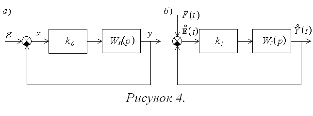
Для расчета
детерминированной составляющей сигнала
ошибки после линеаризации используется
структурная схема (рис. 4,а),
а для расчета центрированной случайной
составляющей — структурная схема (рис.
4,б),
где

=k₁(m_x,σ_x).

Для полученных
структурных схем искомые характеристики
сигнала ошибки определяются следующим
образом: m_E=m_x,
D_E=D_Y.

При расчете
детерминированной составляющей
передаточная функция замкнутой системы
по ошибке имеет вид:

В результате:

.

Среднеквадратическое
отклонение сигнала ошибки в рассматриваемой
задаче полностью определяется возмущающим
воздействием и находится через дисперсию
выходного сигнала и передаточную функцию
замкнутой системы по возмущению, которая
в рассматриваемом примере примет вид:

В результате:

Коэффициенты
полиномов (1) примут вид:

a₀=T₁T₂,

,

,

,
b₀=0,
b₁=0,

.

Определители (3)
будут иметь третий порядок и получаются
следующими:

В результате:

При заданных
k,
T
и c
для расчета характеристик ошибки
необходимо решить систему нелинейных
алгебраических уравнений:

m_E=
,

4. РЕШЕНИЕ УРАВНЕНИЙ
И ПОСТРОЕНИЕ ЗАВИСИМОСТЕЙ

С помощью программы,
написанной на языке MATLAB,
решив систему методом последовательных
приближений, мы найдем зависимости
коэффициентов статистической линеаризации,
математического ожидания и
среднеквадратического отклонения
ошибки системы E(t)
от величины коэффициента передачи k.
Для нахождения зависимости M
от k
использована функция MATLAB
fzero.
Текст программы представлен в приложении
А. Графики зависимостей представлены
на рисунках 5-9.

Рисунок
5

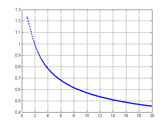
Рисунок 6

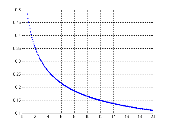
Рисунок 7

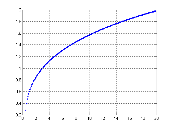
Рисунок 8

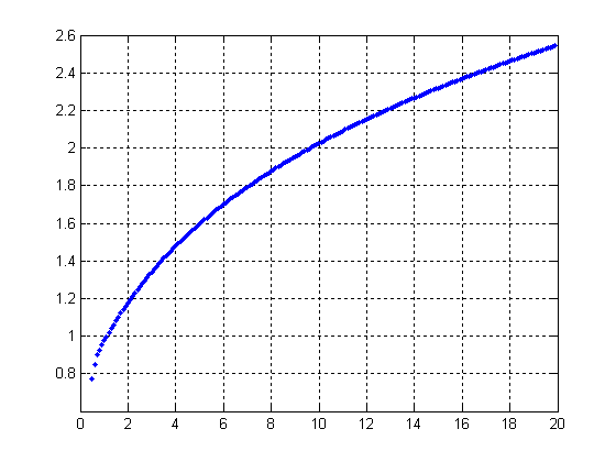
Рисунок 9

Соседние файлы в предмете [НЕСОРТИРОВАННОЕ]

Источник

On Nonidentical Discrete-Time Hyperchaotic Systems Synchronization: Towards Secure Medical Image Transmission

Narjes Khalifa, Mohamed Benrejeb, in Recent Advances in Chaotic Systems and Synchronization, 2019

3.3 Measurement of Encryption and Decryption Quality

Mean Square Error (MSE), Peak Signal-to-Noise Ratio (PSNR), and Structural Similarity Index Measure (SSIM) (see Appendix A) are used to measure the proposed encryption and decryption algorithms quality [51].

In this context, MSE, PSNR, and SSIM are performed between plain and encrypted images, then between plain and decrypted images. The obtained values of SSIM are very close to zero, those of PSNR low, and the MSE ones > 30 dB, which denotes the difference between original and encrypted images, as shown in Table 2.

Table 2. MSE, PSNR, and SSIM Values Between Plain and Encrypted Images

Images	MSE	PSNR	SSIM
Fig. 5A and B	93.2738	8.1372	0.0023
Fig. 5D and E	75.8129	7.7288	0.0041
Fig. 5G and H	42.2462	5.9944	0.0034

Furthermore, for plain and decrypted images, the obtained values of SSIM are very close to 1, those of PSNR high, and MSE values close to 0, as shown in Table 3. As a result, the different resultant values of MSE, PSNR, and SSIM show the effectiveness of the proposed encryption algorithm applied to secure medical image transmission.

Table 3. MSE, PSNR, and SSIM Values Between Plain and Decrypted Images

Images	MSE	PSNR	SSIM
Fig. 5A and C	6.1 × 10^− 5	49.9718	0.9998
Fig. 5D and F	0	55.8007	0.9999
Fig. 5G and I	0	48.9251	0.9995

Read full chapter

URL:

https://www.sciencedirect.com/science/article/pii/B9780128158388000169

Multichannel Image Recovery

Nikolas P. Galatsanos, … Rafael Molina, in Handbook of Image and Video Processing (Second Edition), 2005

3.1 Linear Minimum Mean Square Error (LMMSE) Estimation

The mean square error (MSE), defined as

(4)MSE(fˆ)=E{‖f−fˆ‖2},

is a measure of the quality of the image estimate fˆ. Here, E{·} denotes the expectation operator. Among the images that are a linear function of the data (i.e., fˆ=Ag where A a matrix), the image that minimizes the MSE is known as the linear minimum mean square error (LMMSE) estimate f_LMMSE. Assuming f and n are uncorrelated [4], the LMMSE solution is found by finding the matrix A that minimizes the MSE. The resulting LMMSE solution is

(5)fLMMSE=CfHT(HCfHT+Cn)−1g,

where C_n is the covariance matrix of the multichannel noise vector n, and C_f is the KNM × KNM covariance matrix of the multichannel image vector f, defined as

(6)Cf=E{f fT}=[C11C12…C1KC22C22…C2K…………CK1CK2…CKK],

where Cij=E{fjfiT}.

Using the matrix inversion lemma [14] it is easy to show that

(7)CfHT(HCfH+Cn)−1=(HTCn−1H+Cf−)−1HTCn−1.

Thus, we can also write

(8)fLMMSE=(HTCn−1H+Cf−1)−1HTCn−1g.

Read full chapter

URL:

https://www.sciencedirect.com/science/article/pii/B9780121197926500760

Regression analysis

Kanishka Tyagi, … Michael Manry, in Artificial Intelligence and Machine Learning for EDGE Computing, 2022

3 Cost functions

The cost function is used to understand how close a machine learning model is predicted to the actual output. The cost function is essential and should be the first measure to be chosen while performing machine learning-related tasks. For different applications, different sets of cost functions are used. Cost functions are also called loss functions. Below, we describe the most commonly used cost function and also discuss for which application it is used.

3.1 MSE

Mean square error (MSE) is most widely used in the regression model, where the independent variable that is the target values are continuous. It is measured as the mean squared differences between actual output and predicted output, which is defined as

(2)E=1Nv∑p=1Nv[tp−yp]2

where t_p is the pth pattern of actual output and y_p is the pth pattern of the predicted output. N_v is the total number of patterns. t_p −y_p is also called as residual error. MSE is also called as L2 loss and is said to be less robust to outliers. If there is an outlier in the dataset and as we can see that the residuals are squared, those outliers are doubled, which contributes to larger prediction values which can also result to greater weight changes.

3.2 MSLE

Mean square logarithmic error (MLSE) is similar to MSE. MLSE is preferred when treating both small and large errors equally and does not want large errors to influence training.

(3)E=1Nv∑p=1Nv[log(tp+1)−log(yp+1)]2

From the previous equation, we can observe that “1” is added as log(0) is undefined.

3.3 RMSE

Root mean square error (RMSE) is similar to MSE expect we need to square root the MSE. RMSE behaves like the standard deviation of the residuals, which indicate how spread the residuals are.

(4)E=1Nv∑p=1Nv[tp−yp]2

Similar to MSLE, RMSLE is also a cost function, where we add a log function and add a one to Eq. (4) similar to Eq. (3). RMSE is preferred over MSE when lower residuals are of importance.

3.4 MAE

Mean absolute error (MAE) cost is measured as the mean differences between actual output and predicted output, which is defined as

(5)E=1Nv∑p=1Nv|tp−yp|

where the difference is the absolute value rather than squared as in MSE. MAE is also called as L1 loss and robust to outliers as we do not square the residuals.

Read full chapter

URL:

https://www.sciencedirect.com/science/article/pii/B9780128240540000071

Optimization of Methods for Image-Texture Segmentation Using Ant Colony Optimization

Manasa Nadipally, in Intelligent Data Analysis for Biomedical Applications, 2019

2.4 Evaluation of Segmentation Techniques

Assessment is essential in deciding which segmentation algorithm is suitable to be selected. For extraction of the boundary, the edge detection is assessed by using root-mean-square-error (RMSE), mean-square error (MSE), peak signal-to-noise ratio (PSNR), and signal-to-noise ratio (SNR) [30–32].

2.4.1 Mean-Square Error

MSE value denotes the average difference of the pixels all over the image. A higher value of MSE designates a greater difference amid the original image and processed image. Nonetheless, it is indispensable to be extremely careful with the edges. The following equation provides a formula for calculation of the MSE.

(2.24)MSE=1N∑∑(Eij−oij)2

here, N is the image size, O is the original image, whereas, E is the edge image.

2.4.2 Root-Mean-Square-Error

The RMSE is extensively used for measuring the differences between values forecasted by an estimator, or model, and the values that are observed. The RMSE aggregates the magnitudes of the predictions errors several times into a single distinct measure of predictive power. It is a measure of precision. The RMSE value can be calculated by taking the square root of MSE.

(2.25)RMSE=1N∑∑(Eij−oij)2

2.4.3 Signal-to-Noise Ratio

SNR describes the total noise present in the output edge detected in an image, in comparison to the noise in the original signal level. SNR is a quality metric and presents a rough calculation of the possibility of false switching; it serves as a mean to compare the relative performance of different implementations [33–35]. SNR is estimated by Eq. (2.26):

(2.26)SNR=[ΣiΣj(Eij)2ΣiΣj(Eij−oij)2]

2.4.4 Peak Signal-to-Noise Ratio

The PSNR calculates the PSNR ratio in decibels amid two images. We often use this ratio as a measurement of quality between the original image and the resultant image. The higher the value of PSNR, the better will be the quality of the output image. For calculating the PSNR, MSE is used. We calculate the PSNR by using Eq. (2.27).

(2.27)PSNR=10⋅log10(MAXI2MSE)=20⋅log10(MAXIMSE)=20⋅log10(MAXI)−10⋅log10(MSE)

Here, MAX_I is the maximum possible pixel value of the image

Read full chapter

URL:

https://www.sciencedirect.com/science/article/pii/B9780128155530000021

Uplink Physical Layer Functions

Sassan Ahmadi, in LTE-Advanced, 2014

10.9.5.1 LMMSE receiver

An LMMSE receiver is a widely used solution which generates an MMSE estimate for each time-domain symbol. The MMSE has been used as a baseline receiver in LTE/LTE-Advanced evaluations due to its simplicity. The detection problem in an LMMSE receiver reduces to finding a weighting matrix such that sˆ1(k,l)=W1(k,l)y1(k,l), where the weighting matrix is given as follows [25–27,43,44]:

(10.18)W1(k,l)=Hˆ1H(k,l)R−1;R=P1Hˆ1(k,l)H1H(k,l)+σ2I

where Hˆj(k,l) and σ2 denote the estimated channel matrix and noise power, respectively, P1 is the transmission power of the serving cell and is given by P1=E[|s1(k,l)|2].

Due to the linearity and unitary properties of DFT, an equivalent equalization method would be to obtain a frequency-domain MMSE estimate for each symbol in the frequency-domain, and then take the IDFT to obtain the time-domain MMSE symbol estimation. The MMSE estimation for each frequency-domain symbol is obtained by linearly combining received signals collected from multiple receive antennas in the frequency-domain, using MMSE combining weights W(k)=[H(k)HH(k)+R(k)]–1H(k), where k is the sub-carrier index, H(k) is a vector representing the frequency response for the layer signal of interest (one element per receive antenna), and R(k) is the impairment covariance matrix encompassing the spatial correlation between the impairment components. The performance of this simple MMSE equalizer asymptotically approaches the theoretical capacity in a SIMO channel. However, in a MIMO channel, LMMSE equalizer performance is far from the SIMO capacity due to the presence of spatial multiplexing interference [127].

Read full chapter

URL:

https://www.sciencedirect.com/science/article/pii/B9780124051621000101

Digital Picture Formats and Representations

David R. Bull, in Communicating Pictures, 2014

Peak signal to noise ratio (PSNR)

Mean Square Error-based metrics are in common use as objective measures of distortion, due mainly to their ease of calculation. An image with a higher MSE will generally express more visible distortions than one with a low MSE. In image and video compression, it is however common practice to use Peak Signal to Noise Ratio (PSNR) rather than MSE to characterize reconstructed image quality. PSNR is of particular use if images are being compared with different dynamic ranges and it is employed for a number of different reasons:

1.: MSE values will take on different meanings if the wordlength of the signal samples changes.
2.: Unlike many natural signals, the mean of an image or video frame is not normally zero and indeed will vary from frame to frame.
3.: PSNR normalizes MSE with respect to the peak signal value rather than signal variance, and in doing so enables direct comparison between the results from different codecs or systems.
4.: PSNR can never be less than zero.

The PSNR for our image S is given by:

(4.25)PSNR=10·log10Asmax2∑x=0X-1∑y=0Y-1(e[x,y])2

where for a wordlength B:smax=2B-1. We can also include a binary mask, b[x,y], so that the PSNR value for a specific arbitrary image region can be calculated. Thus:

(4.26)PSNR=10·log10smax2∑x=0X-1∑y=0Y-1b[x,y]∑x=0X-1∑y=0Y-1(e[x,y])2

Although there is no perceptual basis for PSNR, it does fit reasonably well with subjective assessments, especially in cases where algorithms are compared that produce similar types of artifact. It remains the most commonly used objective distortion metric, because of its mathematical tractability and because of the lack of any widely accepted alternative. It is worth noting, however, that PSNR can be deceptive, for example when:

1.: There is a phase shift in the reconstructed signal. Even tiny phase shifts that the human observer would not notice will produce significant changes.
2.: There is visual masking in the coding process that provides perceptually high quality by hiding distortions in regions where they are less noticeable.
3.: Errors persist over time. A single small error in a single frame may not be noticeable, yet it could be annoying if it persists over many frames.
4.: Comparisons are being made between different coding strategies (e.g. synthesis based vs block transform based (see Chapters 10 and 13Chapter 10Chapter 13)).

Consider the images in Figure 4.18. All of these have the same PSNR value (16.5 dB), but most people would agree that they do not exhibit the same perceptual qualities. In particular, the bottom right image with a small spatial shift is practically indistinguishable from the original. In cases such as this, perception-based metrics can offer closer correlation with subjective opinions and these are considered in more detail in Chapter 10.

Example 4.5 Calculating PSNR

Consider a 3×3 image S of 8-bit values and its approximation after compression and reconstruction, S~. Calculate the MSE and the PSNR of the reconstructed block.

Figure 4.18. Quality comparisons for the same PSNR (16.5 dB). Top left to bottom right: original; AWGN (variance 0.24); grid lines; salt and pepper noise; spatial shift by 5 pixels vertically and horizontally.

Solution

We can see that X=3,Y=3,smax=255, and A=9. Using equation (4.22) the MSE is given by:

MSE=79

and from equation (4.25), it can be seen that the PSNR for this block is given by:

PSNR=10·log109×25527=49.2dB

Read full chapter

URL:

https://www.sciencedirect.com/science/article/pii/B9780124059061000040

Energy-Efficient MIMO–OFDM Systems

Zimran Rafique, Boon-Chong Seet, in Handbook of Green Information and Communication Systems, 2013

15.2.1.2.2 MMSE Detection Algorithm

The minimum mean square error (MMSE) detection algorithm has almost the same computational complexity as the ZF detection algorithm but gives more reliable results even with a noisy estimation of the channel due to the introduction of diagonal matrix 1SNRINr in the MMSE filter (G_MMSE) equation [29]. This algorithm consists of following steps with the assumption that channel response “H” is known at the receiver side:

•

Calculate GMMSE=H∗[HH∗+1SNRINr]-1 where 1SNR is the noise power to signal power ratio and INr is the identity matrix of size N_r.

•

Select the ith row of GMMSE and multiply it with Rec to detect the signal yi:

yi=GMMSE̲iRec.

•

The estimated value of the signal is detected by slicing to the nearest value in the signal constellation:

S^i=Q(yi).

Read full chapter

URL:

https://www.sciencedirect.com/science/article/pii/B9780124158443000152

Mean-Square Error Linear Estimation

Sergios Theodoridis, in Machine Learning (Second Edition), 2020

4.1 Introduction

Mean-square error (MSE) linear estimation is a topic of fundamental importance for parameter estimation in statistical learning. Besides historical reasons, which take us back to the pioneering works of Kolmogorov, Wiener, and Kalman, who laid the foundations of the optimal estimation field, understanding MSE estimation is a must, prior to studying more recent techniques. One always has to grasp the basics and learn the classics prior to getting involved with new “adventures.” Many of the concepts to be discussed in this chapter are also used in the next chapters.

Optimizing via a loss function that builds around the square of the error has a number of advantages, such as a single optimal value, which can be obtained via the solution of a linear set of equations; this is a very attractive feature in practice. Moreover, due to the relative simplicity of the resulting equations, the newcomer in the field can get a better feeling of the various notions associated with optimal parameter estimation. The elegant geometric interpretation of the MSE solution, via the orthogonality theorem, is presented and discussed. In the chapter, emphasis is also given to computational complexity issues while solving for the optimal solution. The essence behind these techniques remains exactly the same as that inspiring a number of computationally efficient schemes for online learning, to be discussed later in this book.

The development of the chapter is around real-valued variables, something that will be true for most of the book. However, complex-valued signals are particularly useful in a number of areas, with communications being a typical example, and the generalization from the real to the complex domain may not always be trivial. Although in most of the cases the difference lies in changing matrix transpositions by Hermitian ones, this is not the whole story. This is the reason that we chose to deal with complex-valued data in separate sections, whenever the differences from the real data are not trivial and some subtle issues are involved.

Read full chapter

URL:

https://www.sciencedirect.com/science/article/pii/B9780128188033000131

Accruement of nonlinear dynamical system and its dynamics: electronics and cryptographic engineering

Najeeb Alam Khan, … Tooba Hameed, in Fractional Order Systems and Applications in Engineering, 2023

Mean square error (MSE)

The mean square error (MSE) is calculated to make sure that the original and decrypted images are in variations or not. The lesser the MSE between two images, the better the decryption; it is defined as

MSE(q1,q2)=1MN∑i=0M−1∑j=0N−1(q1(i,j)−q2(i,j))2,

where q1(i,j) and q2(i,j) indicate the original and decrypted images, respectively.

Read full chapter

URL:

https://www.sciencedirect.com/science/article/pii/B9780323909532000153

Detection methods

Yi Hong, … Emanuele Viterbo, in Delay-Doppler Communications, 2022

6.3.3 Complexity

The LMMSE methods of (6.18) and (6.19) in the delay-Doppler domain and time domain, respectively, require inverting an NM×NM matrix, thereby incurring a complexity of O((NM)3). Note that the cubic complexity can be reduced by taking advantage of the banded and sparse structure of H and G, as well as the fact that the time domain matrix G is sparser than H, since |L|⩽P⩽S.

For CP/ZP-OTFS, the LMMSE detection can be performed block-wise for N blocks (see (6.20)), which requires inverting N submatrices of size M×M, followed by transforming the time domain estimates to the delay-Doppler domain. Hence, such detection has an overall complexity of O(NM3+NMlog2⁡N)), which is significantly lower than for the LMMSE methods in (6.18) and (6.19). In addition, the sparsity and banded nature of these submatrices can be exploited to further reduce detection complexity.

Read full chapter

URL:

https://www.sciencedirect.com/science/article/pii/B9780323850285000141

Источник

В статистических данных и обработки сигналов , A минимальной среднеквадратической ошибки ( MMSE ) оценки является метод оценки , который минимизирует среднеквадратичную ошибку (MSE), которая является общей мерой оценки качества, из подогнанных значений зависимой переменной . В байесовской установке термин MMSE более конкретно относится к оценке с квадратичной функцией потерь . В таком случае оценка MMSE задается апостериорным средним значением параметра, который необходимо оценить. Поскольку вычисление апостериорного среднего затруднительно, форма оценки MMSE обычно ограничивается определенным классом функций. Линейные оценщики MMSE — популярный выбор, поскольку они просты в использовании, легко вычисляются и очень универсальны. Это породило множество популярных оценок , таких как фильтр Винера-Колмогорова и фильтра Калмана .

Мотивация

Термин MMSE более конкретно относится к оценке в байесовской среде с квадратичной функцией стоимости. Основная идея байесовского подхода к оценке проистекает из практических ситуаций, когда у нас часто есть некоторая предварительная информация о параметре, который нужно оценить. Например, у нас может быть предварительная информация о диапазоне, который может принимать параметр; или у нас может быть старая оценка параметра, который мы хотим изменить, когда станет доступным новое наблюдение; или статистика фактического случайного сигнала, такого как речь. Это контрастирует с небайесовским подходом, таким как несмещенная оценка с минимальной дисперсией (MVUE), где предполагается, что о параметре заранее ничего не известно и который не учитывает такие ситуации. В байесовском подходе такая априорная информация фиксируется априорной функцией плотности вероятности параметров; и основанный непосредственно на теореме Байеса , он позволяет нам делать более точные апостериорные оценки по мере появления большего количества наблюдений. Таким образом, в отличие от небайесовского подхода, при котором представляющие интерес параметры считаются детерминированными, но неизвестными константами, байесовская оценка стремится оценить параметр, который сам по себе является случайной величиной. Кроме того, байесовская оценка также может иметь дело с ситуациями, когда последовательность наблюдений не обязательно независима. Таким образом, байесовская оценка представляет собой еще одну альтернативу MVUE. Это полезно, когда MVUE не существует или не может быть найден.

Определение

Пусть будет скрытой случайной векторной переменной, и пусть будет известной случайной векторной переменной (измерение или наблюдение), причем обе они не обязательно имеют одинаковую размерность. Оценка по какой — либо функции измерения . Вектор ошибки оценки задается выражением, а его среднеквадратическая ошибка (MSE) задается следом ковариационной матрицы ошибок. Икс Икс

${ displaystyle operatorname {MSE} = operatorname {tr} left { operatorname {E} {({ hat {x}} - x) ({ hat {x}} - x) ^ {T } } right } = operatorname {E} {({ hat {x}} - x) ^ {T} ({ hat {x}} - x) },}$

где ожидание берется за и . Когда — скалярная переменная, выражение MSE упрощается до . Обратите внимание, что MSE может быть эквивалентно определено другими способами, поскольку
Икс Икс ${ displaystyle operatorname {E} left {({ hat {x}} - x) ^ {2} right }}$

${ displaystyle operatorname {tr} left { operatorname {E} {ee ^ {T} } right } = operatorname {E} left { operatorname {tr} {ee ^ { T} } right } = operatorname {E} {e ^ {T} e } = sum _ {i = 1} ^ {n} operatorname {E} {e_ {i} ^ { 2} }.}$

Затем оценщик MMSE определяется как оценщик, достигающий минимальной MSE:

${ displaystyle { hat {x}} _ { operatorname {MMSE}} (y) = operatorname {argmin} _ { hat {x}} operatorname {MSE}.}$

Характеристики

Когда средние значения и дисперсии конечны, оценка MMSE определяется однозначно и определяется следующим образом:

${ displaystyle { hat {x}} _ { operatorname {MMSE}} (y) = operatorname {E} {x mid y }.}$

Другими словами, оценка MMSE — это условное ожидание данного известного наблюдаемого значения измерений. Икс

Оценка MMSE является беспристрастной (согласно предположениям регулярности, упомянутым выше):

${ displaystyle operatorname {E} {{ hat {x}} _ { operatorname {MMSE}} (y) } = operatorname {E} { operatorname {E} {x mid y } } = operatorname {E} {x }.}$

Оценщик MMSE асимптотически несмещен и сходится по распределению к нормальному распределению:

${ sqrt {n}} ({ hat {x}} - x) { xrightarrow {d}} { mathcal {N}} left (0, I ^ {- 1} (x) right),$

где есть информация Фишера из . Таким образом, оценка MMSE асимптотически эффективна . Я (х)

${ displaystyle operatorname {E} {({ hat {x}} _ { operatorname {MMSE}} -x) g (y) } = 0}$

для всех в замкнутом линейном подпространстве измерений. Для случайных векторов, поскольку MSE для оценки случайного вектора является суммой MSE координат, нахождение оценки MMSE для случайного вектора разлагается на нахождение оценок MMSE для координат X по отдельности:
г (г)

${ displaystyle { mathcal {V}} = {g (y) mid g: mathbb {R} ^ {m} rightarrow mathbb {R}, operatorname {E} {g (y) ^ {2} } <+ infty }}$

${ displaystyle operatorname {E} {(g_ {i} ^ {*} (y) -x_ {i}) g_ {j} (y) } = 0,}$

для всех i и j . Говоря более кратко, взаимная корреляция между минимальной ошибкой оценки и средством оценки должна быть равна нулю,
${ displaystyle { hat {x}} _ { operatorname {MMSE}} -x}$

${ displaystyle operatorname {E} {({ hat {x}} _ { operatorname {MMSE}} -x) { hat {x}} ^ {T} } = 0.}$

Линейный оценщик MMSE

Во многих случаях невозможно определить аналитическое выражение оценки MMSE. Два основных численных подхода для получения оценки MMSE зависят либо от нахождения условного ожидания, либо от нахождения минимумов MSE. Прямая численная оценка условного ожидания требует больших вычислительных ресурсов, поскольку часто требует многомерного интегрирования, обычно выполняемого с помощью методов Монте-Карло . Другой вычислительный подход заключается в прямом поиске минимумов MSE с использованием таких методов, как методы стохастического градиентного спуска ; но этот метод по-прежнему требует оценки ожидания. Хотя эти численные методы оказались плодотворными, выражение в закрытой форме для оценки MMSE, тем не менее, возможно, если мы готовы пойти на некоторые компромиссы.

Одна из возможностей состоит в том, чтобы отказаться от требований полной оптимальности и найти метод минимизации MSE в рамках определенного класса оценщиков, такого как класс линейных оценщиков. Таким образом, мы постулируем , что условное математическое ожидание данности является простым линейной функцией , где измерение является случайным вектором, является матрицей и является вектором. Это можно рассматривать как приближение Тейлора первого порядка . Линейный оценщик MMSE — это оценщик, достигающий минимальной MSE среди всех оценщиков такой формы. То есть решает следующие задачи оптимизации:
Икс

${ displaystyle min _ {W, b} operatorname {MSE} qquad { text {st}} qquad { hat {x}} = Wy + b.}$

Одним из преимуществ такого линейного средства оценки MMSE является то, что нет необходимости явно вычислять апостериорную функцию плотности вероятности . Такая линейная оценка зависит только от первых двух моментов и . Таким образом, хотя может быть удобно предположить, что и являются вместе гауссовыми, нет необходимости делать это предположение, пока предполагаемое распределение имеет хорошо определенные первый и второй моменты. Форма линейной оценки не зависит от типа предполагаемого базового распределения.
Икс Икс Икс

Выражение для оптимального и определяется выражением:

$W = C_ {XY} C_ {Y} ^ {- 1}.$

где , является кросс-ковариационная матрица между и , то есть автоматически ковариационная матрица .
$C _ {{XY}}$ Икс $C _ {{Y}}$

Таким образом, выражение для линейной оценки MMSE, его среднего значения и автоковариации имеет вид

{ hat {x}} = W (y - { bar {y}}) + { bar {x}},

{ displaystyle operatorname {E} {{ hat {x}} } = { bar {x}},}

$C _ { hat {X}} = C_ {XY} C_ {Y} ^ {- 1} C_ {YX},$

где — матрица кросс-ковариации между и .
$C _ {{YX}}$ Икс

Наконец, ковариация ошибки и минимальная среднеквадратичная ошибка, достижимые такой оценкой, равны

$C_ {e} = C_ {X} -C _ { hat {X}} = C_ {X} -C_ {XY} C_ {Y} ^ {- 1} C_ {YX},$

${ displaystyle operatorname {LMMSE} = operatorname {tr} {C_ {e} }.}$

Вывод по принципу ортогональности

Пусть у нас есть оптимальная линейная оценка MMSE, заданная как , где мы должны найти выражение для и . Требуется, чтобы оценка MMSE была беспристрастной. Это означает,

{ displaystyle operatorname {E} {{ hat {x}} } = operatorname {E} {x }.}

Подставляя выражение для выше, мы получаем

где и . Таким образом, мы можем переписать оценку как

и выражение для ошибки оценки принимает вид

{ hat {x}} - x = W (y - { bar {y}}) - (x - { bar {x}}).

Исходя из принципа ортогональности, мы можем иметь , где возьмем . Здесь левый член
${ displaystyle operatorname {E} {({ hat {x}} - x) (y - { bar {y}}) ^ {T} } = 0}$

${ displaystyle { begin {align} operatorname {E} {({ hat {x}} - x) (y - { bar {y}}) ^ {T} } & = operatorname {E } {(W (y - { bar {y}}) - (x - { bar {x}})) (y - { bar {y}}) ^ {T} } \ & = W operatorname {E} {(y - { bar {y}}) (y - { bar {y}}) ^ {T} } - operatorname {E} {(x - { bar {x}}) (y - { bar {y}}) ^ {T} } \ & = WC_ {Y} -C_ {XY}. end {выровнено}}}$

Приравнивая к нулю, мы получаем искомое выражение для as

${ displaystyle W = C_ {XY} C_ {Y} ^ {- 1}.}$

Является кросс-ковариационная матрица между Х и Y, а это автоматически ковариационная матрица Y. Так , выражение может быть также переписана в терминах , как
$C _ {{XY}}$ $C _ {{Y}}$ $C_ {XY} = C_ {YX} ^ {T}$ $C _ {{YX}}$

${ displaystyle W ^ {T} = C_ {Y} ^ {- 1} C_ {YX}.}$

Таким образом, полное выражение для линейной оценки MMSE имеет вид

${ displaystyle { hat {x}} = C_ {XY} C_ {Y} ^ {- 1} (y - { bar {y}}) + { bar {x}}.}$

Поскольку оценка сама по себе является случайной величиной с , мы также можем получить ее автоковариацию как

${ displaystyle { begin {align} C _ { hat {X}} & = operatorname {E} {({ hat {x}} - { bar {x}}) ({ hat {x} } - { bar {x}}) ^ {T} } \ & = W operatorname {E} {(y - { bar {y}}) (y - { bar {y}}) ^ {T} } W ^ {T} \ & = WC_ {Y} W ^ {T}. \ конец {выровнен}}}$

Подставляя выражение для и , получаем
$W ^ {T}$

$C _ { hat {X}} = C_ {XY} C_ {Y} ^ {- 1} C_ {YX}.$

Наконец, ковариация линейной ошибки оценки MMSE будет тогда выражена как

${ displaystyle { begin {align} C_ {e} & = operatorname {E} {({ hat {x}} - x) ({ hat {x}} - x) ^ {T} } \ & = operatorname {E} {({ hat {x}} - x) (W (y - { bar {y}}) - (x - { bar {x}})) ^ { T} } \ & = underbrace { operatorname {E} {({ hat {x}} - x) (y - { bar {y}}) ^ {T} }} _ {0 } W ^ {T} - operatorname {E} {({ hat {x}} - x) (x - { bar {x}}) ^ {T} } \ & = - operatorname { E} {(W (y - { bar {y}}) - (x - { bar {x}})) (x - { bar {x}}) ^ {T} } \ & = operatorname {E} {(x - { bar {x}}) (x - { bar {x}}) ^ {T} } - W operatorname {E} {(y - { bar {y}}) (x - { bar {x}}) ^ {T} } \ & = C_ {X} -WC_ {YX}. end {align}}}$

Первый член в третьей строке равен нулю из-за принципа ортогональности. Поскольку мы можем переписать в терминах ковариационных матриц как
$W = C_ {XY} C_ {Y} ^ {- 1}$ $C_ {e}$

$C_ {e} = C_ {X} -C_ {XY} C_ {Y} ^ {- 1} C_ {YX}.$

Мы можем признать, что это то же самое, что и. Таким образом, минимальная среднеквадратичная ошибка, достижимая такой линейной оценкой, равна
$C_ {e} = C_ {X} -C _ { hat {X}}.$

${ displaystyle operatorname {LMMSE} = operatorname {tr} {C_ {e} }}$

Одномерный случай

Для особого случая, когда оба и являются скалярами, приведенные выше отношения упрощаются до
Икс

${ displaystyle { hat {x}} = { frac { sigma _ {XY}} { sigma _ {Y} ^ {2}}} (y - { bar {y}}) + { bar {x}} = rho { frac { sigma _ {X}} { sigma _ {Y}}} (y - { bar {y}}) + { bar {x}},}$

${ displaystyle sigma _ {e} ^ {2} = sigma _ {X} ^ {2} - { frac { sigma _ {XY} ^ {2}} { sigma _ {Y} ^ {2 }}} = (1- rho ^ {2}) sigma _ {X} ^ {2},}$

где — коэффициент корреляции Пирсона между и .
rho Икс

Вычисление

Стандартный метод, такой как исключение Гаусса, может использоваться для решения матричного уравнения для . Более стабильный в числовом отношении метод обеспечивается методом QR-разложения . Поскольку матрица является симметричной положительно определенной матрицей, ее можно решить в два раза быстрее с помощью разложения Холецкого , в то время как для больших разреженных систем метод сопряженных градиентов более эффективен. Рекурсия Левинсона — это быстрый метод, когда она также является матрицей Теплица . Это может произойти, когда это стационарный процесс в широком смысле . В таких стационарных случаях эти оценки также называют фильтрами Винера – Колмогорова .
$C_ {Y}$ $C_ {Y}$

Линейная оценка MMSE для процесса линейного наблюдения

Давайте далее смоделируем основной процесс наблюдения как линейный процесс:, где — известная матрица, а — вектор случайного шума со средним значением и кросс-ковариацией . Здесь искомое среднее и ковариационные матрицы будут
$C_ {XZ} = 0$

{ displaystyle operatorname {E} {y } = A { bar {x}},}

$C_ {Y} = AC_ {X} A ^ {T} + C_ {Z},$

$C_ {XY} = C_ {X} A ^ {T}.$

Таким образом, выражение для матрицы линейной оценки MMSE дополнительно изменяется на

$W = C_ {X} A ^ {T} (AC_ {X} A ^ {T} + C_ {Z}) ^ {- 1}.$

Подставляя все в выражение для , получаем

${ hat {x}} = C_ {X} A ^ {T} (AC_ {X} A ^ {T} + C_ {Z}) ^ {- 1} (yA { bar {x}}) + { bar {x}}.$

Наконец, ковариация ошибок равна

$C_ {e} = C_ {X} -C _ { hat {X}} = C_ {X} -C_ {X} A ^ {T} (AC_ {X} A ^ {T} + C_ {Z}) ^ {-1} AC_ {X}.$

Существенное различие между описанной выше задачей оценивания и проблемой наименьших квадратов и оценкой Гаусса-Маркова состоит в том, что количество наблюдений m (т. Е. Размерность ) не обязательно должно быть по крайней мере таким же большим, как количество неизвестных n (т. Е. размер ). Оценка для процесса линейного наблюдения существует при условии, что M матрицы с размерностью м матрица существует; это так для любого m, если, например, положительно определено. Физическая причина этого свойства заключается в том, что, поскольку теперь это случайная величина, можно сформировать значимую оценку (а именно ее среднее значение) даже без измерений. Каждое новое измерение просто предоставляет дополнительную информацию, которая может изменить нашу первоначальную оценку. Еще одна особенность этой оценки состоит в том, что при m < n погрешности измерения быть не должно. Таким образом, мы можем иметь , потому что, пока она положительно определена, оценка все еще существует. Наконец, этот метод может обрабатывать случаи, когда шум коррелирован.
Икс $(AC_ {X} A ^ {T} + C_ {Z}) ^ {- 1}$ $C_ {Z}$ Икс $C_ {Z} = 0$ $AC_ {X} A ^ {T}$

Альтернативная форма

Альтернативная форма выражения может быть получена с помощью матричного тождества

$C_ {X} A ^ {T} (AC_ {X} A ^ {T} + C_ {Z}) ^ {- 1} = (A ^ {T} C_ {Z} ^ {- 1} A + C_ { X} ^ {- 1}) ^ {- 1} A ^ {T} C_ {Z} ^ {- 1},$

что может быть установлено путем последующего умножения на и предварительного умножения на, чтобы получить
$(AC_ {X} A ^ {T} + C_ {Z})$ $(A ^ {T} C_ {Z} ^ {- 1} A + C_ {X} ^ {- 1}),$

$W = (A ^ {T} C_ {Z} ^ {- 1} A + C_ {X} ^ {- 1}) ^ {- 1} A ^ {T} C_ {Z} ^ {- 1},$

а также

$C_ {e} = (A ^ {T} C_ {Z} ^ {- 1} A + C_ {X} ^ {- 1}) ^ {- 1}.$

Поскольку теперь можно записать в терминах as , мы получаем упрощенное выражение для as
$C_ {e}$ $W = C_ {e} A ^ {T} C_ {Z} ^ {- 1}$

${ hat {x}} = C_ {e} A ^ {T} C_ {Z} ^ {- 1} (yA { bar {x}}) + { bar {x}}.$

В таком виде приведенное выше выражение легко сравнить с взвешенным методом наименьших квадратов и оценкой Гаусса – Маркова . В частности, когда , соответствующий бесконечной дисперсии априорной информации относительно , результат идентичен взвешенной линейной оценке по методу наименьших квадратов с использованием весовой матрицы. Более того, если компоненты не коррелированы и имеют одинаковую дисперсию, так что где — единичная матрица, то она идентична обычной оценке методом наименьших квадратов.
$C_ {X} ^ {- 1} = 0$ Икс $W = (A ^ {T} C_ {Z} ^ {- 1} A) ^ {- 1} A ^ {T} C_ {Z} ^ {- 1}$ $C_ {Z} ^ {- 1}$ $C_ {Z} = sigma ^ {2} I,$ $W = (A ^ {T} A) ^ {- 1} A ^ {T}$

Последовательная линейная оценка MMSE

Во многих приложениях реального времени данные наблюдений недоступны в виде единого пакета. Вместо этого наблюдения производятся последовательно. Наивное применение предыдущих формул заставило бы нас отбросить старую оценку и пересчитать новую оценку по мере поступления свежих данных. Но тогда мы теряем всю информацию, предоставленную старым наблюдением. Когда наблюдения являются скалярными величинами, один из возможных способов избежать таких повторных вычислений — сначала объединить всю последовательность наблюдений, а затем применить стандартную формулу оценки, как это сделано в Примере 2. Но это может быть очень утомительно, поскольку количество наблюдений увеличивается, поэтому увеличивается размер матриц, которые необходимо инвертировать и умножать. Также этот метод трудно распространить на случай векторных наблюдений. Другой подход к оценке на основе последовательных наблюдений — просто обновить старую оценку по мере появления дополнительных данных, что приведет к более точным оценкам. Таким образом, желателен рекурсивный метод, при котором новые измерения могут изменять старые оценки. В этих обсуждениях подразумевается предположение, что статистические свойства не меняются со временем. Другими словами, стационарен.
Икс Икс

Для последовательной оценки, если у нас есть оценка, основанная на измерениях, генерирующих пространство , то после получения другого набора измерений мы должны вычесть из этих измерений ту часть, которую можно было бы ожидать по результатам первых измерений. Другими словами, обновление должно быть основано на той части новых данных, которая ортогональна старым данным.
${ hat {x}} _ {1}$ $Г_ {1}$

Предположим, что оптимальная оценка была сформирована на основе прошлых измерений и что матрица ковариации ошибок равна . Для процессов линейного наблюдения наилучшей оценкой, основанной на прошлых наблюдениях и, следовательно, старой оценке , является . Вычитая из , получаем ошибку предсказания
${ hat {x}} _ {1}$ $C_ {e_ {1}}$ ${ hat {x}} _ {1}$ ${ hat {y}} = А { hat {x}} _ {1}$

${ tilde {y}} = y - { hat {y}} = A (x - { hat {x}} _ {1}) + z = Ae_ {1} + z$

Новая оценка, основанная на дополнительных данных, теперь

${ hat {x}} _ {2} = { hat {x}} _ {1} + C_ {X { tilde {Y}}} C _ { tilde {Y}} ^ {- 1} { тильда {y}},$

где — кросс-ковариация между и и — автоковариация $C_ {X { tilde {Y}}}$ Икс $C _ { tilde {Y}}$

Используя тот факт, что и , мы можем получить ковариационные матрицы в терминах ковариации ошибок как
$х = { hat {x}} _ {1} + e_ {1}$

$C _ { tilde {Y}} = AC_ {e_ {1}} A ^ {T} + C_ {Z},$

${ displaystyle C_ {X { tilde {Y}}} = operatorname {E} {({ hat {x}} _ {1} + e_ {1} - { bar {x}}) (Ae_ {1} + z) ^ {T} } = C_ {e_ {1}} A ^ {T}.}$

Собирая все вместе, мы получаем новую оценку как

${ hat {x}} _ {2} = { hat {x}} _ {1} + C_ {e_ {1}} A ^ {T} (AC_ {e_ {1}} A ^ {T} + C_ {Z}) ^ {- 1} (yA { hat {x}} _ {1}),$

и новая ковариация ошибок как

$C_ {e_ {2}} = C_ {e_ {1}} - C_ {e_ {1}} A ^ {T} (AC_ {e_ {1}} A ^ {T} + C_ {Z}) ^ {- 1} AC_ {e_ {1}}.$

Повторное использование двух вышеупомянутых уравнений по мере того, как становится доступным больше наблюдений, приводит к методам рекурсивной оценки. Более компактно выражения можно записать как

${ displaystyle K_ {t + 1} = C_ {e_ {t}} A ^ {T} (AC_ {e_ {t}} A ^ {T} + C_ {Z}) ^ {- 1},}$
${ displaystyle { hat {x}} _ {t + 1} = { hat {x}} _ {t} + K_ {t + 1} (yA { hat {x}} _ {t}), }$
${ displaystyle C_ {e_ {t + 1}} = (I-K_ {t + 1} A) C_ {e_ {t}}.}$

Матрицу часто называют коэффициентом усиления. Повторение этих трех шагов по мере того, как становится доступным больше данных, приводит к итерационному алгоритму оценки. Обобщение этой идеи на нестационарные случаи приводит к созданию фильтра Калмана . Три этапа обновления, описанные выше, действительно образуют этап обновления фильтра Калмана.

Частный случай: скалярные наблюдения

В качестве важного частного случая может быть получено простое в использовании рекурсивное выражение, когда в каждый t-й момент времени основной процесс линейного наблюдения выдает скаляр, такой что , где — известный вектор-столбец размером n на 1, значения которого могут изменяться со временем , представляет собой оцениваемый случайный вектор-столбец размером n на 1 и представляет собой скалярный шумовой член с дисперсией . После ( t +1) -го наблюдения прямое использование приведенных выше рекурсивных уравнений дает выражение для оценки как:
${ displaystyle y_ {t} = a_ {t} ^ {T} x_ {t} + z_ {t}}$ $x_ {t}$ $z_ {t}$ $sigma _ {t} ^ {2}$ ${ displaystyle { hat {x}} _ {t + 1}}$

${ displaystyle { hat {x}} _ {t + 1} = { hat {x}} _ {t} + k_ {t + 1} (y_ {t + 1} -a_ {t + 1} ^ {T} { hat {x}} _ {t})}$

где это новое наблюдение скалярного и коэффициент усиления является п его-1 вектор — столбца задается
${ displaystyle y_ {t + 1}}$ $к_ {т + 1}$

${ Displaystyle к_ {т + 1} = { гидроразрыва {(С_ {е}) _ {т} а_ {т + 1}} { sigma _ {т + 1} ^ {2} + а_ {т + 1 } ^ {T} (C_ {e}) _ {t} a_ {t + 1}}}.}$

Является п матрицы с размерностью п ошибка ковариационная матрица задается
${ displaystyle (C_ {e}) _ {t + 1}}$

${ displaystyle (C_ {e}) _ {t + 1} = (I-k_ {t + 1} a_ {t + 1} ^ {T}) (C_ {e}) _ {t}.}$

Здесь инверсия матрицы не требуется. Кроме того, коэффициент усиления зависит от нашей уверенности в новой выборке данных, измеренной по дисперсии шума, по сравнению с предыдущими данными. За начальные значения и принимаются среднее значение и ковариация априорной функции плотности вероятности .
$к_ {т + 1}$ $C_ {e}$ Икс

Альтернативные подходы: этот важный частный случай также привел к появлению многих других итерационных методов (или адаптивных фильтров ), таких как фильтр наименьших средних квадратов и рекурсивный фильтр наименьших квадратов , которые напрямую решают исходную проблему оптимизации MSE с использованием стохастических градиентных спусков . Однако, поскольку ошибку оценки нельзя непосредственно наблюдать, эти методы пытаются минимизировать среднеквадратичную ошибку прогноза . Например, в случае скалярных наблюдений у нас есть градиент. Таким образом, уравнение обновления для фильтра наименьших квадратов имеет вид
${ displaystyle mathrm {E} {{ tilde {y}} ^ {T} { tilde {y}} }}$ ${ displaystyle nabla _ { hat {x}} mathrm {E} {{ tilde {y}} ^ {2} } = - 2 mathrm {E} {{ tilde {y}} а }.}$

${ displaystyle { hat {x}} _ {t + 1} = { hat {x}} _ {t} + eta _ {t} mathrm {E} {{ tilde {y}} _ {t} a_ {t} },}$

где — размер скалярного шага, а математическое ожидание аппроксимируется мгновенным значением . Как мы видим, эти методы обходят необходимость в ковариационных матрицах.
${ displaystyle eta _ {t}}$ ${ displaystyle mathrm {E} {a_ {t} { tilde {y}} _ {t} } приблизительно a_ {t} { tilde {y}} _ {t}}$

Примеры

Пример 1

В качестве примера возьмем задачу линейного прогнозирования . Пусть линейная комбинация наблюдаемых скалярных случайных величин и будет использоваться для оценки другой будущей скалярной случайной величины, такой что . Если случайные величины являются действительными гауссовскими случайными величинами с нулевым средним и ее ковариационная матрица, заданная формулой
${ displaystyle z_ {1}, z_ {2}}$ ${ displaystyle z_ {3}}$ ${ displaystyle z_ {4}}$ ${ displaystyle { hat {z}} _ {4} = sum _ {i = 1} ^ {3} w_ {i} z_ {i}}$ ${ displaystyle z = [z_ {1}, z_ {2}, z_ {3}, z_ {4}] ^ {T}}$

${ displaystyle operatorname {cov} (Z) = operatorname {E} [zz ^ {T}] = left [{ begin {array} {cccc} 1 & 2 & 3 & 4 \ 2 & 5 & 8 & 9 \ 3 & 8 & 6 & 10 \ 4 & 9 & 10 & 15 end { массив}} right],}$

то наша задача — найти такие коэффициенты , чтобы получить оптимальную линейную оценку .
$w_ {i}$ ${ displaystyle { hat {z}} _ {4}}$

В терминах терминологии, разработанной в предыдущих разделах, для этой задачи у нас есть вектор наблюдения , матрица оценки как вектор-строка и оцениваемая переменная как скалярная величина. Матрица автокорреляции определяется как
${ Displaystyle у = [z_ {1}, z_ {2}, z_ {3}] ^ {T}}$ $Ш = [ш_ {1}, ш_ {2}, ш_ {3}]$ ${ displaystyle x = z_ {4}}$ $C_ {Y}$

${ Displaystyle C_ {Y} = left [{ begin {array} {ccc} E [z_ {1}, z_ {1}] & E [z_ {2}, z_ {1}] и E [z_ {3} , z_ {1}] \ E [z_ {1}, z_ {2}] & E [z_ {2}, z_ {2}] & E [z_ {3}, z_ {2}] \ E [z_ { 1}, z_ {3}] & E [z_ {2}, z_ {3}] & E [z_ {3}, z_ {3}] end {array}} right] = left [{ begin {array } {ccc} 1 & 2 & 3 \ 2 & 5 & 8 \ 3 & 8 & 6 end {array}} right].}$

Матрица взаимной корреляции определяется как
$C _ {{YX}}$

${ Displaystyle C_ {YX} = left [{ begin {array} {c} E [z_ {4}, z_ {1}] \ E [z_ {4}, z_ {2}] \ E [ z_ {4}, z_ {3}] end {array}} right] = left [{ begin {array} {c} 4 \ 9 \ 10 end {array}} right].}$

Теперь мы решаем уравнение путем инвертирования и предварительного умножения, чтобы получить
$C_ {Y} W ^ {T} = C_ {YX}$ $C_ {Y}$

${ displaystyle C_ {Y} ^ {- 1} C_ {YX} = left [{ begin {array} {ccc} 4.85 & -1.71 & -0.142 \ - 1.71 & 0.428 & 0.2857 \ - 0.142 & 0 .2857 & -0,1429 end {array}} right] left [{ begin {array} {c} 4 \ 9 \ 10 end {array}} right] = left [{ begin {array } {c} 2,57 \ - 0,142 \ 0,5714 end {array}} right] = W ^ {T}.}$

Итак, у нас есть и
в качестве оптимальных коэффициентов для . Тогда вычисление минимальной среднеквадратичной ошибки дает . Обратите внимание, что нет необходимости получать явную матрицу, обратную для вычисления значения . Матричное уравнение может быть решено с помощью хорошо известных методов, таких как метод исключения Гаусса. Более короткий нечисловой пример можно найти в принципе ортогональности .
${ displaystyle w_ {1} = 2,57,}$ ${ displaystyle w_ {2} = - 0,142,}$ $w _ {{3}} =. 5714$ ${ displaystyle { hat {z}} _ {4}}$ ${ displaystyle left Vert e right Vert _ { min} ^ {2} = operatorname {E} [z_ {4} z_ {4}] - WC_ {YX} = 15-WC_ {YX} = .2857}$ $C_ {Y}$

Пример 2

Рассмотрим вектор, сформированный путем наблюдений за фиксированным, но неизвестным скалярным параметром, нарушенным белым гауссовским шумом. Мы можем описать процесс линейным уравнением , где . В зависимости от контекста будет ясно, представляет ли он скаляр или вектор. Предположим, что мы знаем, что это диапазон, в который будет попадать значение. Мы можем смоделировать нашу неопределенность с помощью априорного равномерного распределения по интервалу и, таким образом, будем иметь дисперсию . Пусть вектор шума распределен нормально, как где — единичная матрица. Также и независимы и . Легко увидеть, что
Икс $1 = [1,1, ldots, 1] ^ {T}$ $[-x_ {0}, x_ {0}]$ Икс Икс $[-x_ {0}, x_ {0}]$ Икс $sigma _ {X} ^ {2} = x_ {0} ^ {2} / 3.$ $N (0, sigma _ {Z} ^ {2} I)$ Икс $C_ {XZ} = 0$

${ displaystyle { begin {align} & operatorname {E} {y } = 0, \ & C_ {Y} = operatorname {E} {yy ^ {T} } = sigma _ {X } ^ {2} 11 ^ {T} + sigma _ {Z} ^ {2} I, \ & C_ {XY} = operatorname {E} {xy ^ {T} } = sigma _ {X } ^ {2} 1 ^ {T}. End {выравнивается}}}$

Таким образом, линейная оценка MMSE имеет вид

${ begin {align} { hat {x}} & = C_ {XY} C_ {Y} ^ {- 1} y \ & = sigma _ {X} ^ {2} 1 ^ {T} ( sigma _ {X} ^ {2} 11 ^ {T} + sigma _ {Z} ^ {2} I) ^ {- 1} y. end {выровнено}}$

Мы можем упростить выражение, используя альтернативную форму для as

${ displaystyle { begin {align} { hat {x}} & = left (1 ^ {T} { frac {1} { sigma _ {Z} ^ {2}}} I1 + { frac { 1} { sigma _ {X} ^ {2}}} right) ^ {- 1} 1 ^ {T} { frac {1} { sigma _ {Z} ^ {2}}} Iy \ & = { frac {1} { sigma _ {Z} ^ {2}}} left ({ frac {N} { sigma _ {Z} ^ {2}}} + { frac {1} { sigma _ {X} ^ {2}}} right) ^ {- 1} 1 ^ {T} y \ & = { frac { sigma _ {X} ^ {2}} { sigma _ {X} ^ {2} + sigma _ {Z} ^ {2} / N}} { bar {y}}, end {align}}}$

где у нас есть $y = [y_ {1}, y_ {2}, ldots, y_ {N}] ^ {T}$ ${ bar {y}} = { frac {1 ^ {T} y} {N}} = { frac { sum _ {i = 1} ^ {N} y_ {i}} {N}}.$

Точно так же дисперсия оценки равна

$sigma _ { hat {X}} ^ {2} = C_ {XY} C_ {Y} ^ {- 1} C_ {YX} = { Big (} { frac { sigma _ {X} ^ { 2}} { sigma _ {X} ^ {2} + sigma _ {Z} ^ {2} / N}} { Big)} sigma _ {X} ^ {2}.$

Таким образом, MMSE этой линейной оценки

${ displaystyle operatorname {LMMSE} = sigma _ {X} ^ {2} - sigma _ { hat {X}} ^ {2} = { Big (} { frac { sigma _ {Z} ^ {2}} { sigma _ {X} ^ {2} + sigma _ {Z} ^ {2} / N}} { Big)} { frac { sigma _ {X} ^ {2} } {N}}.}$

Для очень больших мы видим, что оценка MMSE скаляра с равномерным априорным распределением может быть аппроксимирована средним арифметическим всех наблюдаемых данных.

${ displaystyle { hat {x}} = { frac {1} {N}} sum _ {i = 1} ^ {N} y_ {i},}$

в то время как дисперсия не будет зависеть от данных, и LMMSE оценки будет стремиться к нулю.
$sigma _ { hat {X}} ^ {2} = sigma _ {X} ^ {2},$

Однако оценка является неоптимальной, поскольку ограничена линейностью. Если бы случайная величина также была гауссовой, тогда оценка была бы оптимальной. Обратите внимание, что форма оценки останется неизменной, независимо от априорного распределения , до тех пор, пока среднее и дисперсия этих распределений одинаковы.
Икс Икс

Пример 3

Рассмотрим вариант приведенного выше примера: на выборах баллотируются два кандидата. Пусть доля голосов , что кандидат получит на день выборов будет Таким образом доля голосов, другой кандидат получит будет Примем как случайная величина с равномерным априорное распределение , так что его среднее значение и дисперсия Несколько За несколько недель до выборов два независимых опроса общественного мнения провели два независимых опроса общественного мнения. Первый опрос показал, что кандидат, скорее всего, наберет небольшую часть голосов. Так как некоторые ошибки всегда присутствует из — за конечной выборки и методологии частности опроса , принятого, первый опросчик объявляет свою оценку , чтобы иметь ошибку с нулевым средним и дисперсией Аналогично, второй опросчик объявляет свою оценку , чтобы быть с ошибкой с нулевым средним и дисперсией Обратите внимание, что, за исключением среднего значения и дисперсии ошибки, распределение ошибок не указано. Как следует объединить эти два опроса, чтобы получить прогноз голосования для данного кандидата?
1-х. Икс [0,1] $sigma _ {X} ^ {2} = 1/12.$ $г_ {1}$ $z_ {1}$ $sigma _ {Z_ {1}} ^ {2}.$ $г_ {2}$ $z_ {2}$ $sigma _ {Z_ {2}} ^ {2}.$

Как и в предыдущем примере, у нас есть

${ begin {выравнивается} y_ {1} & = x + z_ {1} \ y_ {2} & = x + z_ {2}. end {выравнивается}}$

Здесь оба файла . Таким образом, мы можем получить оценку LMMSE как линейную комбинацию и как
${ displaystyle operatorname {E} {y_ {1} } = operatorname {E} {y_ {2} } = { bar {x}} = 1/2}$ $г_ {1}$ $г_ {2}$

${ hat {x}} = w_ {1} (y_ {1} - { bar {x}}) + w_ {2} (y_ {2} - { bar {x}}) + { bar { Икс}},$

где веса даны как

${ begin {align} w_ {1} & = { frac {1 / sigma _ {Z_ {1}} ^ {2}} {1 / sigma _ {Z_ {1}} ^ {2} +1 / sigma _ {Z_ {2}} ^ {2} + 1 / sigma _ {X} ^ {2}}}, \ w_ {2} & = { frac {1 / sigma _ {Z_ { 2}} ^ {2}} {1 / sigma _ {Z_ {1}} ^ {2} + 1 / sigma _ {Z_ {2}} ^ {2} + 1 / sigma _ {X} ^ {2}}}. End {выравнивается}}$

Здесь, поскольку член знаменателя постоянен, опросу с меньшей ошибкой дается более высокий вес, чтобы предсказать результат выборов. Наконец, дисперсия прогноза определяется выражением

$sigma _ { hat {X}} ^ {2} = { frac {1 / sigma _ {Z_ {1}} ^ {2} + 1 / sigma _ {Z_ {2}} ^ {2} } {1 / sigma _ {Z_ {1}} ^ {2} + 1 / sigma _ {Z_ {2}} ^ {2} + 1 / sigma _ {X} ^ {2}}} sigma _ {X} ^ {2},$

что делает меньше, чем $sigma _ { hat {X}} ^ {2}$ $sigma _ {X} ^ {2}.$

В общем, если у нас есть опросчики, то где вес для i-го опроса определяется как ${ displaystyle { hat {x}} = sum _ {i = 1} ^ {N} w_ {i} (y_ {i} - { bar {x}}) + { bar {x}}, }$ ${ displaystyle w_ {i} = { frac {1 / sigma _ {Z_ {i}} ^ {2}} { sum _ {i = 1} ^ {N} 1 / sigma _ {Z_ {i }} ^ {2} + 1 / sigma _ {X} ^ {2}}}.}$

Пример 4

Предположим, что музыкант играет на инструменте, и звук улавливается двумя микрофонами, каждый из которых расположен в двух разных местах. Пусть ослабление звука из-за расстояния до каждого микрофона равно и , которые считаются известными константами. Аналогично, пусть шум на каждом микрофоне будет и , каждый с нулевым средним значением и дисперсией и соответственно. Позвольте обозначить звук, издаваемый музыкантом, который является случайной величиной с нулевым средним значением и дисперсией. Как следует объединить записанную музыку с этих двух микрофонов после синхронизации друг с другом?
$а_ {1}$ $а_ {2}$ $z_ {1}$ $z_ {2}$ $sigma _ {Z_ {1}} ^ {2}$ $sigma _ {Z_ {2}} ^ {2}$ Икс $sigma _ {X} ^ {2}.$

Мы можем смоделировать звук, получаемый каждым микрофоном, как

${ begin {align} y_ {1} & = a_ {1} x + z_ {1} \ y_ {2} & = a_ {2} x + z_ {2}. end {выравнивается}}$

Здесь оба файла . Таким образом, мы можем объединить два звука как
${ displaystyle operatorname {E} {y_ {1} } = operatorname {E} {y_ {2} } = 0}$

$y = w_ {1} y_ {1} + w_ {2} y_ {2}$

где i-й вес задается как

$w_ {i} = { frac {a_ {i} / sigma _ {Z_ {i}} ^ {2}} { sum _ {i} a_ {i} ^ {2} / sigma _ {Z_ { i}} ^ {2} + 1 / sigma _ {X} ^ {2}}}.$

Смотрите также

Байесовская оценка
Среднеквадратичная ошибка
Наименьших квадратов
Несмещенная оценка с минимальной дисперсией (MVUE)
Принцип ортогональности
Фильтр Винера
Фильтр Калмана
Линейное предсказание
Эквалайзер с нулевым форсированием

Примечания

^
«Среднеквадратичная ошибка (MSE)» . www.probabilitycourse.com . Дата обращения 9 мая 2017 .
^ Мун и Стирлинг.

дальнейшее чтение

Джонсон, Д. «Оценщики минимальной среднеквадратичной ошибки» . Связи. Архивировано из минимальных среднеквадратичных оценщиков ошибок оригинала 25 июля 2008 года . Проверено 8 января 2013 года .
Джейнс, ET (2003). Теория вероятностей: логика науки . Издательство Кембриджского университета. ISBN 978-0521592710.
Bibby, J .; Тутенбург, Х. (1977). Прогнозирование и улучшенная оценка в линейных моделях . Вайли. ISBN 9780471016564.
Lehmann, EL; Казелла, Г. (1998). «Глава 4». Теория точечного оценивания (2-е изд.). Springer. ISBN 0-387-98502-6.
Кей, С.М. (1993). Основы статистической обработки сигналов: теория оценивания . Прентис Холл. стр. 344 -350. ISBN 0-13-042268-1.
Люенбергер, Д.Г. (1969). «Глава 4, Оценка методом наименьших квадратов». Оптимизация методами векторного пространства (1-е изд.). Вайли. ISBN 978-0471181170.
Луна, ТЗ; Стирлинг, WC (2000). Математические методы и алгоритмы обработки сигналов (1-е изд.). Прентис Холл. ISBN 978-0201361865.
Ван Trees, HL (1968). Выявление, оценка и теория модуляции, часть I . Нью-Йорк: Вили. ISBN 0-471-09517-6.
Хайкин, СО (2013). Теория адаптивного фильтра (5-е изд.). Прентис Холл. ISBN 978-0132671453.

Источник

При использовании
критерия минимума СКО, взвешивающие коэффициенты ячеек эквалайзера подстраиваются
так, чтобы минимизировать средний квадрат ошибки

, (10.2.24)

где — информационный символ,
переданный на -ом
сигнальном интервале, a — оценка этого символа на выходе
эквалайзера, определяемая (10.2.1). Если информационные символы комплексные, то
показатель качества при СКО критерия, обозначаемый , определяется так

. (10.2.25)

С другой стороны, когда
информационные символы вещественные, показатель качества просто равен квадрату
вещественной величины . В любом случае, является квадратичнйй
функцией коэффициентов эквалайзера . При дальнейшем обсуждении мы
рассмотрим минимизацию комплексной формы, даваемой (10.2.25).

Эквалайзер неограниченной
длины. Сначала
определим взвешивающие коэффициенты ячеек, которые минимизируют , когда эквалайзер
имеет неограниченное число ячеек. В этом случае, оценка определяется так

(10.2.26)

Подстановка (10.2.26) в
выражение для ,
определяемая (10.2.25), и расширение результата приводит к квадратичной функции
от коэффициентов .
Эту функцию можно легко минимизировать по посредством решения системы
(неограниченной) линейных уравнений для . Альтернативно, систему линейных
уравнений можно получить путём использования принципа ортогональности при
среднеквадратичном оценивании. Это значит, мы выбираем коэффициенты такие, что ошибка ортогональна
сигнальной

последовательности для . То есть

(10.2.27)

Подстановка в (10.2.27) даёт

или, что эквивалентно,

. (10.2.28)

Чтобы вычислить моменты в
(10.2.28), мы используем выражение для даваемое (10.1.16). Таким образом,
получим

(10.2.29)

(10.2.30)

Теперь, если подставим
(10.2.29) и (10.2.30) в (10.2.28) и возьмём -преобразование от обеих частей
результирующего уравнения, мы находим

. (10.2.31)

Следовательно,
передаточная функция эквалайзера, основанного на критерии минимума СКО, равна

. (10.2.32)

Если обеляющий фильтр
включён в ,
мы получаем эквивалентный эквалайзер с передаточной функцией

. (10.2.33)

Видим, что единственная
разница между этим выражением для и тем, которое базируется на критерии
пикового искажения — это спектральная плотность шума , которая появилась в (10.2.33),
Если очень
мало по сравнению с сигналом, коэффициенты, которые минимизируют пиковые
искажения приближённо
равны коэффициентам, которые минимизируют по СКО показатель качества . Это значит, что в
пределе, когда ,
два критерия дают одинаковое решение для взвешивающих коэффициентов. Следовательно,
когда , минимизация
СКО ведёт к полному исключению МСИ. С другой стороны, это не так, когда . В общем, когда , оба критерия дают
остаточное МСИ и аддитивный шум на выходе эквалайзера.

Меру остаточного МСИ и
аддитивного шума на выходе эквалайзера можно получить расчётом минимальной
величины ,
обозначаемую ,
когда передаточная функция

эквалайзера определена
(10.2.32). Поскольку и поскольку с учётом условия
ортогональности (10.2.27), следует

. (10.2.34)

Эта частная форма для не очень
информативна. Больше понимания зависимости качества эквалайзера от канальных
характеристик можно получить, если суммы в (10.2.34) преобразовать в частотную
область. Это можно выполнить, заметив, что сумма в (10.2.34) является свёрткой и , вычисленной при
нулевом сдвиге. Так, если через обозначить свёртку этих
последовательностей, то сумма в (10.2.34) просто равна . Поскольку — преобразование
последовательности равно

, (10.2.35)

то слагаемое равно

. (10.2.36)

Контурный интеграл в
(10.2.36) можно преобразовать в эквивалентный линейный интеграл путём замены
переменной .
В результате этой замены получаем

. (10.2.37)

Наконец, подставив (10.2.37)
в сумму (10.2.34), получаем желательное выражение для минимума СКО в виде

(10.2.38)

В отсутствие МСИ и, следовательно,

. (10.2.39)

Видим, что . Далее,
соотношение между выходным (нормированного по энергии сигнала) ОСШ и выглядит так

Более
существенно то, что соотношение и также имеет силу, когда имеется
остаточная МСИ в дополнении к шуму на выходе эквалайзера.

Эквалайзер ограниченной длины. Теперь
вернём наше внимание к случаю, когда длительность импульсной характеристики
трансверсального эквалайзера простирается на ограниченном временном интервале,
т.е. эквалайзер имеет конечную память или ограниченную длину. Выход эквалайзера
на -м сигнальном
интервале равен

СКО эквалайзера с ячейками, обозначаемый , равен

Минимизация по взвешивающим
коэффициентам ячеек или, что эквивалентно, требуя, чтобы
ошибка была
бы ортогональна сигнальным отсчётам , , приводит к следующей системе
уравнений:

где

Удобно
выразить систему линейных уравнений в матричной форме, т.е.

где означает вектор столбец взвешивающих
значений кодовых ячеек, означает матрицу ковариаций Эрмита с
элементами ;
а мерный
вектор столбец с элементами . Решение (10.2.46) можно записать в
виде

Таким образом, решение для включает в себя
обращение матрицы . Оптимальные взвешивающие
коэффициенты ячеек, даваемые (10.2.47), минимизируют показатель качества , что приводит к
минимальной величине

где определяет транспонированный вектор
столбец .
можно
использовать в (10.2.40) для вычисления ОСШ линейного эквивалента с коэффициентами
ячеек.

In statistics and signal processing, a minimum mean square error (MMSE) estimator is an estimation method which minimizes the mean square error (MSE), which is a common measure of estimator quality, of the fitted values of a dependent variable. In the Bayesian setting, the term MMSE more specifically refers to estimation with quadratic loss function. In such case, the MMSE estimator is given by the posterior mean of the parameter to be estimated. Since the posterior mean is cumbersome to calculate, the form of the MMSE estimator is usually constrained to be within a certain class of functions. Linear MMSE estimators are a popular choice since they are easy to use, easy to calculate, and very versatile. It has given rise to many popular estimators such as the Wiener–Kolmogorov filter and Kalman filter.

Motivation[edit]

The term MMSE more specifically refers to estimation in a Bayesian setting with quadratic cost function. The basic idea behind the Bayesian approach to estimation stems from practical situations where we often have some prior information about the parameter to be estimated. For instance, we may have prior information about the range that the parameter can assume; or we may have an old estimate of the parameter that we want to modify when a new observation is made available; or the statistics of an actual random signal such as speech. This is in contrast to the non-Bayesian approach like minimum-variance unbiased estimator (MVUE) where absolutely nothing is assumed to be known about the parameter in advance and which does not account for such situations. In the Bayesian approach, such prior information is captured by the prior probability density function of the parameters; and based directly on Bayes theorem, it allows us to make better posterior estimates as more observations become available. Thus unlike non-Bayesian approach where parameters of interest are assumed to be deterministic, but unknown constants, the Bayesian estimator seeks to estimate a parameter that is itself a random variable. Furthermore, Bayesian estimation can also deal with situations where the sequence of observations are not necessarily independent. Thus Bayesian estimation provides yet another alternative to the MVUE. This is useful when the MVUE does not exist or cannot be found.

Definition[edit]

Let be a hidden random vector variable, and let be a known random vector variable (the measurement or observation), both of them not necessarily of the same dimension. An estimator of is any function of the measurement . The estimation error vector is given by and its mean squared error (MSE) is given by the trace of error covariance matrix

${displaystyle operatorname {MSE} =operatorname {tr} left{operatorname {E} {({hat {x}}-x)({hat {x}}-x)^{T}}right}=operatorname {E} {({hat {x}}-x)^{T}({hat {x}}-x)},}$

where the expectation is taken over conditioned on . When is a scalar variable, the MSE expression simplifies to ${displaystyle operatorname {E} left{({hat {x}}-x)^{2}right}}$ . Note that MSE can equivalently be defined in other ways, since

${displaystyle operatorname {tr} left{operatorname {E} {ee^{T}}right}=operatorname {E} left{operatorname {tr} {ee^{T}}right}=operatorname {E} {e^{T}e}=sum _{i=1}^{n}operatorname {E} {e_{i}^{2}}.}$

The MMSE estimator is then defined as the estimator achieving minimal MSE:

${displaystyle {hat {x}}_{operatorname {MMSE} }(y)=operatorname {argmin} _{hat {x}}operatorname {MSE} .}$

Properties[edit]

When the means and variances are finite, the MMSE estimator is uniquely defined^[1] and is given by:

${displaystyle {hat {x}}_{operatorname {MMSE} }(y)=operatorname {E} {xmid y}.}$

In other words, the MMSE estimator is the conditional expectation of

given the known observed value of the measurements. Also, since ${displaystyle {hat {x}}_{mathrm {MMSE} }}$ is the posterior mean, the error covariance matrix $C_{e}$ is equal to the posterior covariance ${displaystyle C_{X|Y}}$ matrix,

${displaystyle C_{e}=C_{X|Y}}$ .

The MMSE estimator is unbiased (under the regularity assumptions mentioned above):

${displaystyle operatorname {E} {{hat {x}}_{operatorname {MMSE} }(y)}=operatorname {E} {operatorname {E} {xmid y}}=operatorname {E} {x}.}$

The MMSE estimator is asymptotically unbiased and it converges in distribution to the normal distribution:

${displaystyle {sqrt {n}}({hat {x}}_{operatorname {MMSE} }-x)xrightarrow {d} {mathcal {N}}left(0,I^{-1}(x)right),}$

where

is the Fisher information of

. Thus, the MMSE estimator is asymptotically efficient.

${displaystyle operatorname {E} {({hat {x}}_{operatorname {MMSE} }-x)g(y)}=0}$

for all

in closed, linear subspace ${displaystyle {mathcal {V}}={g(y)mid g:mathbb {R} ^{m}rightarrow mathbb {R} ,operatorname {E} {g(y)^{2}}<+infty }}$

of the measurements. For random vectors, since the MSE for estimation of a random vector is the sum of the MSEs of the coordinates, finding the MMSE estimator of a random vector decomposes into finding the MMSE estimators of the coordinates of X separately:

${displaystyle operatorname {E} {(g_{i}^{*}(y)-x_{i})g_{j}(y)}=0,}$

for all i and j. More succinctly put, the cross-correlation between the minimum estimation error ${displaystyle {hat {x}}_{operatorname {MMSE} }-x}$ and the estimator

should be zero,

${displaystyle operatorname {E} {({hat {x}}_{operatorname {MMSE} }-x){hat {x}}^{T}}=0.}$

Linear MMSE estimator[edit]

In many cases, it is not possible to determine the analytical expression of the MMSE estimator. Two basic numerical approaches to obtain the MMSE estimate depends on either finding the conditional expectation or finding the minima of MSE. Direct numerical evaluation of the conditional expectation is computationally expensive since it often requires multidimensional integration usually done via Monte Carlo methods. Another computational approach is to directly seek the minima of the MSE using techniques such as the stochastic gradient descent methods ; but this method still requires the evaluation of expectation. While these numerical methods have been fruitful, a closed form expression for the MMSE estimator is nevertheless possible if we are willing to make some compromises.

One possibility is to abandon the full optimality requirements and seek a technique minimizing the MSE within a particular class of estimators, such as the class of linear estimators. Thus, we postulate that the conditional expectation of given is a simple linear function of , , where the measurement is a random vector, is a matrix and is a vector. This can be seen as the first order Taylor approximation of . The linear MMSE estimator is the estimator achieving minimum MSE among all estimators of such form. That is, it solves the following the optimization problem:

${displaystyle min _{W,b}operatorname {MSE} qquad {text{s.t.}}qquad {hat {x}}=Wy+b.}$

One advantage of such linear MMSE estimator is that it is not necessary to explicitly calculate the posterior probability density function of . Such linear estimator only depends on the first two moments of and . So although it may be convenient to assume that and are jointly Gaussian, it is not necessary to make this assumption, so long as the assumed distribution has well defined first and second moments. The form of the linear estimator does not depend on the type of the assumed underlying distribution.

The expression for optimal and is given by:

$W=C_{XY}C_{Y}^{-1}.$

where , the $C_{{XY}}$ is cross-covariance matrix between and , the $C_{{Y}}$ is auto-covariance matrix of .

Thus, the expression for linear MMSE estimator, its mean, and its auto-covariance is given by

${displaystyle {hat {x}}=C_{XY}C_{Y}^{-1}(y-{bar {y}})+{bar {x}},}$

$C_{hat {X}}=C_{XY}C_{Y}^{-1}C_{YX},$

where the $C_{{YX}}$ is cross-covariance matrix between and .

Lastly, the error covariance and minimum mean square error achievable by such estimator is

$C_{e}=C_{X}-C_{hat {X}}=C_{X}-C_{XY}C_{Y}^{-1}C_{YX},$

${displaystyle operatorname {LMMSE} =operatorname {tr} {C_{e}}.}$

Univariate case[edit]

For the special case when both and are scalars, the above relations simplify to

${displaystyle {hat {x}}={frac {sigma _{XY}}{sigma _{Y}^{2}}}(y-{bar {y}})+{bar {x}}=rho {frac {sigma _{X}}{sigma _{Y}}}(y-{bar {y}})+{bar {x}},}$

${displaystyle sigma _{e}^{2}=sigma _{X}^{2}-{frac {sigma _{XY}^{2}}{sigma _{Y}^{2}}}=(1-rho ^{2})sigma _{X}^{2},}$

where ${displaystyle rho ={frac {sigma _{XY}}{sigma _{X}sigma _{Y}}}}$ is the Pearson’s correlation coefficient between and .

The above two equations allows us to interpret the correlation coefficient either as normalized slope of linear regression

${displaystyle left({frac {{hat {x}}-{bar {x}}}{sigma _{X}}}right)=rho left({frac {y-{bar {y}}}{sigma _{Y}}}right)}$

or as square root of the ratio of two variances

${displaystyle rho ^{2}={frac {sigma _{X}^{2}-sigma _{e}^{2}}{sigma _{X}^{2}}}={frac {sigma _{hat {X}}^{2}}{sigma _{X}^{2}}}}$

When rho =0 , we have and ${displaystyle sigma _{e}^{2}=sigma _{X}^{2}}$ . In this case, no new information is gleaned from the measurement which can decrease the uncertainty in . On the other hand, when , we have ${displaystyle {hat {x}}={frac {sigma _{XY}}{sigma _{Y}}}(y-{bar {y}})+{bar {x}}}$ and ${displaystyle sigma _{e}^{2}=0}$ . Here is completely determined by , as given by the equation of straight line.

Computation[edit]

Standard method like Gauss elimination can be used to solve the matrix equation for . A more numerically stable method is provided by QR decomposition method. Since the matrix $C_{Y}$ is a symmetric positive definite matrix, can be solved twice as fast with the Cholesky decomposition, while for large sparse systems conjugate gradient method is more effective. Levinson recursion is a fast method when $C_{Y}$ is also a Toeplitz matrix. This can happen when is a wide sense stationary process. In such stationary cases, these estimators are also referred to as Wiener–Kolmogorov filters.

Linear MMSE estimator for linear observation process[edit]

Let us further model the underlying process of observation as a linear process: y=Ax+z , where is a known matrix and is random noise vector with the mean and cross-covariance $C_{XZ}=0$ . Here the required mean and the covariance matrices will be

$C_{Y}=AC_{X}A^{T}+C_{Z},$

$C_{XY}=C_{X}A^{T}.$

Thus the expression for the linear MMSE estimator matrix further modifies to

$W=C_{X}A^{T}(AC_{X}A^{T}+C_{Z})^{-1}.$

Putting everything into the expression for , we get

${hat {x}}=C_{X}A^{T}(AC_{X}A^{T}+C_{Z})^{-1}(y-A{bar {x}})+{bar {x}}.$

Lastly, the error covariance is

$C_{e}=C_{X}-C_{hat {X}}=C_{X}-C_{X}A^{T}(AC_{X}A^{T}+C_{Z})^{-1}AC_{X}.$

The significant difference between the estimation problem treated above and those of least squares and Gauss–Markov estimate is that the number of observations m, (i.e. the dimension of ) need not be at least as large as the number of unknowns, n, (i.e. the dimension of ). The estimate for the linear observation process exists so long as the m-by-m matrix $(AC_{X}A^{T}+C_{Z})^{-1}$ exists; this is the case for any m if, for instance, $C_{Z}$ is positive definite. Physically the reason for this property is that since is now a random variable, it is possible to form a meaningful estimate (namely its mean) even with no measurements. Every new measurement simply provides additional information which may modify our original estimate. Another feature of this estimate is that for m < n, there need be no measurement error. Thus, we may have $C_{Z}=0$ , because as long as $AC_{X}A^{T}$ is positive definite, the estimate still exists. Lastly, this technique can handle cases where the noise is correlated.

Alternative form[edit]

An alternative form of expression can be obtained by using the matrix identity

$C_{X}A^{T}(AC_{X}A^{T}+C_{Z})^{-1}=(A^{T}C_{Z}^{-1}A+C_{X}^{-1})^{-1}A^{T}C_{Z}^{-1},$

which can be established by post-multiplying by $(AC_{X}A^{T}+C_{Z})$ and pre-multiplying by $(A^{T}C_{Z}^{-1}A+C_{X}^{-1}),$ to obtain

$W=(A^{T}C_{Z}^{-1}A+C_{X}^{-1})^{-1}A^{T}C_{Z}^{-1},$

and

$C_{e}=(A^{T}C_{Z}^{-1}A+C_{X}^{-1})^{-1}.$

Since can now be written in terms of $C_{e}$ as $W=C_{e}A^{T}C_{Z}^{-1}$ , we get a simplified expression for as

${hat {x}}=C_{e}A^{T}C_{Z}^{-1}(y-A{bar {x}})+{bar {x}}.$

In this form the above expression can be easily compared with weighed least square and Gauss–Markov estimate. In particular, when $C_{X}^{-1}=0$ , corresponding to infinite variance of the apriori information concerning , the result $W=(A^{T}C_{Z}^{-1}A)^{-1}A^{T}C_{Z}^{-1}$ is identical to the weighed linear least square estimate with $C_{Z}^{-1}$ as the weight matrix. Moreover, if the components of are uncorrelated and have equal variance such that $C_{Z}=sigma ^{2}I,$ where is an identity matrix, then $W=(A^{T}A)^{-1}A^{T}$ is identical to the ordinary least square estimate.

Sequential linear MMSE estimation[edit]

In many real-time applications, observational data is not available in a single batch. Instead the observations are made in a sequence. One possible approach is to use the sequential observations to update an old estimate as additional data becomes available, leading to finer estimates. One crucial difference between batch estimation and sequential estimation is that sequential estimation requires an additional Markov assumption.

In the Bayesian framework, such recursive estimation is easily facilitated using Bayes’ rule. Given observations, $y_{1},ldots ,y_{k}$ , Bayes’ rule gives us the posterior density of as

${displaystyle {begin{aligned}p(x|y_{1},ldots ,y_{k})&propto p(y_{k}|x,y_{1},ldots ,y_{k-1})p(x|y_{1},ldots ,y_{k-1})&=p(y_{k}|x)p(x|y_{1},ldots ,y_{k-1}).end{aligned}}}$

The ${displaystyle p(x|y_{1},ldots ,y_{k})}$ is called the posterior density, ${displaystyle p(y_{k}|x)}$ is called the likelihood function, and ${displaystyle p(x|y_{1},ldots ,y_{k-1})}$ is the prior density of k-th time step. Note that the prior density for k-th time step is the posterior density of (k-1)-th time step. This structure allows us to formulate a recursive approach to estimation. Here we have assumed the conditional independence of $y_{k}$ from previous observations ${displaystyle y_{1},ldots ,y_{k-1}}$ given as

${displaystyle p(y_{k}|x,y_{1},ldots ,y_{k-1})=p(y_{k}|x).}$

This is the Markov assumption.

The MMSE estimate $hat{x}_k$ given the th observation is then the mean of the posterior density ${displaystyle p(x|y_{1},ldots ,y_{k})}$ . Here, we have implicitly assumed that the statistical properties of does not change with time. In other words, is stationary.

In the context of linear MMSE estimator, the formula for the estimate will have the same form as before. However, the mean and covariance matrices of and will need to be replaced by those of the prior density ${displaystyle p(x|y_{1},ldots ,y_{k-1})}$ and likelihood ${displaystyle p(y_{k}|x)}$ , respectively.

The mean and covariance matrix of the prior density ${displaystyle p(x|y_{1},ldots ,y_{k-1})}$ is given by the previous MMSE estimate, ${displaystyle {bar {x}}_{k-1}={hat {x}}_{k-1}}$ , and the error covariance matrix,

${displaystyle C_{X|Y_{1},ldots ,Y_{k-1}}=mathrm {E} [(x-{hat {x}}_{k-1})(x-{hat {x}}_{k-1})^{T}]=C_{e_{k-1}},}$

respectively, as per by the property of MMSE estimators.

Similarly, for the linear observation process, the mean and covariance matrix of the likelihood ${displaystyle p(y_{k}|x)}$ is given by ${displaystyle {bar {y}}_{k}=A{hat {x}}_{k-1}}$ and

${displaystyle {begin{aligned}C_{Y_{k}|X}&=mathrm {E} [(y_{k}-{bar {y}}_{k})(y_{k}-{bar {y}}_{k})^{T}]&=mathrm {E} [(A(x-{bar {x}}_{k-1})+z)(A(x-{bar {x}}_{k-1})+z)^{T}]&=AC_{e_{k-1}}A^{T}+C_{Z}.end{aligned}}}$

The difference between the predicted value of $y_{k}$ , as given by ${displaystyle {bar {y}}_{k}=A{hat {x}}_{k-1}}$ , and the observed value of $y_{k}$ gives the prediction error ${displaystyle {tilde {y}}_{k}=y_{k}-{bar {y}}_{k}}$ , which is also referred to as innovation. It is more convenient to represent the linear MMSE in terms of the prediction error, whose mean and covariance are ${displaystyle mathrm {E} [{tilde {y}}_{k}]=0}$ and

${displaystyle C_{{tilde {Y}}_{k}}=C_{Y_{k}|X}}$ .

Hence, in the estimate update formula, we should replace and $C_{X}$ by ${displaystyle {hat {x}}_{k-1}}$ and ${displaystyle C_{e_{k-1}}}$ , respectively. Also, we should replace and $C_{Y}$ by ${displaystyle {bar {y}}_{k-1}}$ and ${displaystyle C_{{tilde {Y}}_{k}}}$ . Lastly, we replace $C_{{XY}}$ by

${displaystyle {begin{aligned}C_{e_{k-1}{tilde {Y}}_{k}}&=mathrm {E} [(x-{hat {x}}_{k-1})(y_{k}-{bar {y}}_{k})^{T}]&=mathrm {E} [(x-{hat {x}}_{k-1})(A(x-{hat {x}}_{k-1})+z)^{T}]&=C_{e_{k-1}}A^{T}.end{aligned}}}$

Thus, we have the new estimate as

${displaystyle {begin{aligned}{hat {x}}_{k}&={hat {x}}_{k-1}+C_{e_{k-1}{tilde {Y}}_{k}}C_{{tilde {Y}}_{k}}^{-1}(y_{k}-{bar {y}}_{k})&={hat {x}}_{k-1}+C_{e_{k-1}}A^{T}(AC_{e_{k-1}}A^{T}+C_{Z})^{-1}(y_{k}-A{hat {x}}_{k-1})end{aligned}}}$

and the new error covariance as

${displaystyle C_{e_{k}}=C_{e_{k-1}}-C_{e_{k-1}}A^{T}(AC_{e_{k-1}}A^{T}+C_{Z})^{-1}AC_{e_{k-1}}.}$

From the point of view of linear algebra, for sequential estimation, if we have an estimate ${hat {x}}_{1}$ based on measurements generating space $Y_{1}$ , then after receiving another set of measurements, we should subtract out from these measurements that part that could be anticipated from the result of the first measurements. In other words, the updating must be based on that part of the new data which is orthogonal to the old data.

The repeated use of the above two equations as more observations become available lead to recursive estimation techniques. The expressions can be more compactly written as

${displaystyle W_{k}=C_{e_{k-1}}A^{T}(AC_{e_{k-1}}A^{T}+C_{Z})^{-1},}$

${displaystyle {hat {x}}_{k}={hat {x}}_{k-1}+W_{k}(y_{k}-A{hat {x}}_{k-1}),}$

${displaystyle C_{e_{k}}=(I-W_{k}A)C_{e_{k-1}}.}$

The matrix $W_{k}$ is often referred to as the Kalman gain factor. The alternative formulation of the above algorithm will give

${displaystyle C_{e_{k}}^{-1}=C_{e_{k-1}}^{-1}+A^{T}C_{Z}^{-1}A,}$

${displaystyle W_{k}=C_{e_{k}}A^{T}C_{Z}^{-1},}$

${displaystyle {hat {x}}_{k}={hat {x}}_{k-1}+W_{k}(y_{k}-A{hat {x}}_{k-1}),}$

The repetition of these three steps as more data becomes available leads to an iterative estimation algorithm. The generalization of this idea to non-stationary cases gives rise to the Kalman filter. The three update steps outlined above indeed form the update step of the Kalman filter.

Special case: scalar observations[edit]

As an important special case, an easy to use recursive expression can be derived when at each k-th time instant the underlying linear observation process yields a scalar such that ${displaystyle y_{k}=a_{k}^{T}x_{k}+z_{k}}$ , where $a_{k}$ is n-by-1 known column vector whose values can change with time, $x_{k}$ is n-by-1 random column vector to be estimated, and $z_{k}$ is scalar noise term with variance . After (k+1)-th observation, the direct use of above recursive equations give the expression for the estimate $hat{x}_{k+1}$ as:

${displaystyle {hat {x}}_{k+1}={hat {x}}_{k}+w_{k+1}(y_{k+1}-a_{k+1}^{T}{hat {x}}_{k})}$

where $y_{{k+1}}$ is the new scalar observation and the gain factor $w_{k+1}$ is n-by-1 column vector given by

${displaystyle w_{k+1}={frac {C_{e_{k}}a_{k+1}}{sigma _{k+1}^{2}+a_{k+1}^{T}C_{e_{k}}a_{k+1}}}.}$

The ${displaystyle C_{e_{k+1}}}$ is n-by-n error covariance matrix given by

${displaystyle C_{e_{k+1}}=(I-w_{k+1}a_{k+1}^{T})C_{e_{k}}.}$

Here, no matrix inversion is required. Also, the gain factor, $w_{k+1}$ , depends on our confidence in the new data sample, as measured by the noise variance, versus that in the previous data. The initial values of and $C_{e}$ are taken to be the mean and covariance of the aprior probability density function of .

Alternative approaches: This important special case has also given rise to many other iterative methods (or adaptive filters), such as the least mean squares filter and recursive least squares filter, that directly solves the original MSE optimization problem using stochastic gradient descents. However, since the estimation error cannot be directly observed, these methods try to minimize the mean squared prediction error ${displaystyle mathrm {E} {{tilde {y}}^{T}{tilde {y}}}}$ . For instance, in the case of scalar observations, we have the gradient ${displaystyle nabla _{hat {x}}mathrm {E} {{tilde {y}}^{2}}=-2mathrm {E} {{tilde {y}}a}.}$ Thus, the update equation for the least mean square filter is given by

${displaystyle {hat {x}}_{k+1}={hat {x}}_{k}+eta _{k}mathrm {E} {{tilde {y}}_{k}a_{k}},}$

where $eta _{k}$ is the scalar step size and the expectation is approximated by the instantaneous value ${displaystyle mathrm {E} {a_{k}{tilde {y}}_{k}}approx a_{k}{tilde {y}}_{k}}$ . As we can see, these methods bypass the need for covariance matrices.

Examples[edit]

Example 1[edit]

We shall take a linear prediction problem as an example. Let a linear combination of observed scalar random variables ${displaystyle z_{1},z_{2}}$ and ${displaystyle z_{3}}$ be used to estimate another future scalar random variable ${displaystyle z_{4}}$ such that ${displaystyle {hat {z}}_{4}=sum _{i=1}^{3}w_{i}z_{i}}$ . If the random variables ${displaystyle z=[z_{1},z_{2},z_{3},z_{4}]^{T}}$ are real Gaussian random variables with zero mean and its covariance matrix given by

${displaystyle operatorname {cov} (Z)=operatorname {E} [zz^{T}]=left[{begin{array}{cccc}1&2&3&42&5&8&93&8&6&104&9&10&15end{array}}right],}$

then our task is to find the coefficients $w_{i}$ such that it will yield an optimal linear estimate ${displaystyle {hat {z}}_{4}}$ .

In terms of the terminology developed in the previous sections, for this problem we have the observation vector ${displaystyle y=[z_{1},z_{2},z_{3}]^{T}}$ , the estimator matrix $W=[w_{1},w_{2},w_{3}]$ as a row vector, and the estimated variable ${displaystyle x=z_{4}}$ as a scalar quantity. The autocorrelation matrix $C_{Y}$ is defined as

${displaystyle C_{Y}=left[{begin{array}{ccc}E[z_{1},z_{1}]&E[z_{2},z_{1}]&E[z_{3},z_{1}]E[z_{1},z_{2}]&E[z_{2},z_{2}]&E[z_{3},z_{2}]E[z_{1},z_{3}]&E[z_{2},z_{3}]&E[z_{3},z_{3}]end{array}}right]=left[{begin{array}{ccc}1&2&32&5&83&8&6end{array}}right].}$

The cross correlation matrix $C_{{YX}}$ is defined as

${displaystyle C_{YX}=left[{begin{array}{c}E[z_{4},z_{1}]E[z_{4},z_{2}]E[z_{4},z_{3}]end{array}}right]=left[{begin{array}{c}4910end{array}}right].}$

We now solve the equation $C_{Y}W^{T}=C_{YX}$ by inverting $C_{Y}$ and pre-multiplying to get

${displaystyle C_{Y}^{-1}C_{YX}=left[{begin{array}{ccc}4.85&-1.71&-0.142-1.71&0.428&0.2857-0.142&0.2857&-0.1429end{array}}right]left[{begin{array}{c}4910end{array}}right]=left[{begin{array}{c}2.57-0.142.5714end{array}}right]=W^{T}.}$

So we have ${displaystyle w_{1}=2.57,}$ ${displaystyle w_{2}=-0.142,}$ and $w_{{3}}=.5714$
as the optimal coefficients for ${displaystyle {hat {z}}_{4}}$ . Computing the minimum
mean square error then gives ${displaystyle leftVert erightVert _{min }^{2}=operatorname {E} [z_{4}z_{4}]-WC_{YX}=15-WC_{YX}=.2857}$ .^[2] Note that it is not necessary to obtain an explicit matrix inverse of $C_{Y}$ to compute the value of . The matrix equation can be solved by well known methods such as Gauss elimination method. A shorter, non-numerical example can be found in orthogonality principle.

Example 2[edit]

Consider a vector formed by taking observations of a fixed but unknown scalar parameter disturbed by white Gaussian noise. We can describe the process by a linear equation y=1x+z , where $1=[1,1,ldots ,1]^{T}$ . Depending on context it will be clear if represents a scalar or a vector. Suppose that we know $[-x_{0},x_{0}]$ to be the range within which the value of is going to fall in. We can model our uncertainty of by an aprior uniform distribution over an interval $[-x_{0},x_{0}]$ , and thus will have variance of $sigma _{X}^{2}=x_{0}^{2}/3.$ . Let the noise vector be normally distributed as $N(0,sigma _{Z}^{2}I)$ where is an identity matrix. Also and are independent and $C_{XZ}=0$ . It is easy to see that

${displaystyle {begin{aligned}&operatorname {E} {y}=0,&C_{Y}=operatorname {E} {yy^{T}}=sigma _{X}^{2}11^{T}+sigma _{Z}^{2}I,&C_{XY}=operatorname {E} {xy^{T}}=sigma _{X}^{2}1^{T}.end{aligned}}}$

Thus, the linear MMSE estimator is given by

${begin{aligned}{hat {x}}&=C_{XY}C_{Y}^{-1}y&=sigma _{X}^{2}1^{T}(sigma _{X}^{2}11^{T}+sigma _{Z}^{2}I)^{-1}y.end{aligned}}$

We can simplify the expression by using the alternative form for as

${displaystyle {begin{aligned}{hat {x}}&=left(1^{T}{frac {1}{sigma _{Z}^{2}}}I1+{frac {1}{sigma _{X}^{2}}}right)^{-1}1^{T}{frac {1}{sigma _{Z}^{2}}}Iy&={frac {1}{sigma _{Z}^{2}}}left({frac {N}{sigma _{Z}^{2}}}+{frac {1}{sigma _{X}^{2}}}right)^{-1}1^{T}y&={frac {sigma _{X}^{2}}{sigma _{X}^{2}+sigma _{Z}^{2}/N}}{bar {y}},end{aligned}}}$

where for $y=[y_{1},y_{2},ldots ,y_{N}]^{T}$ we have ${bar {y}}={frac {1^{T}y}{N}}={frac {sum _{i=1}^{N}y_{i}}{N}}.$

Similarly, the variance of the estimator is

$sigma _{hat {X}}^{2}=C_{XY}C_{Y}^{-1}C_{YX}={Big (}{frac {sigma _{X}^{2}}{sigma _{X}^{2}+sigma _{Z}^{2}/N}}{Big )}sigma _{X}^{2}.$

Thus the MMSE of this linear estimator is

${displaystyle operatorname {LMMSE} =sigma _{X}^{2}-sigma _{hat {X}}^{2}={Big (}{frac {sigma _{Z}^{2}}{sigma _{X}^{2}+sigma _{Z}^{2}/N}}{Big )}{frac {sigma _{X}^{2}}{N}}.}$

For very large , we see that the MMSE estimator of a scalar with uniform aprior distribution can be approximated by the arithmetic average of all the observed data

${displaystyle {hat {x}}={frac {1}{N}}sum _{i=1}^{N}y_{i},}$

while the variance will be unaffected by data $sigma _{hat {X}}^{2}=sigma _{X}^{2},$ and the LMMSE of the estimate will tend to zero.

However, the estimator is suboptimal since it is constrained to be linear. Had the random variable also been Gaussian, then the estimator would have been optimal. Notice, that the form of the estimator will remain unchanged, regardless of the apriori distribution of , so long as the mean and variance of these distributions are the same.

Example 3[edit]

Consider a variation of the above example: Two candidates are standing for an election. Let the fraction of votes that a candidate will receive on an election day be Thus the fraction of votes the other candidate will receive will be 1-x. We shall take as a random variable with a uniform prior distribution over [0,1] so that its mean is and variance is $sigma _{X}^{2}=1/12.$ A few weeks before the election, two independent public opinion polls were conducted by two different pollsters. The first poll revealed that the candidate is likely to get $y_{1}$ fraction of votes. Since some error is always present due to finite sampling and the particular polling methodology adopted, the first pollster declares their estimate to have an error $z_{1}$ with zero mean and variance $sigma _{Z_{1}}^{2}.$ Similarly, the second pollster declares their estimate to be $y_{2}$ with an error $z_{2}$ with zero mean and variance $sigma _{Z_{2}}^{2}.$ Note that except for the mean and variance of the error, the error distribution is unspecified. How should the two polls be combined to obtain the voting prediction for the given candidate?

As with previous example, we have

${begin{aligned}y_{1}&=x+z_{1}y_{2}&=x+z_{2}.end{aligned}}$

Here, both the ${displaystyle operatorname {E} {y_{1}}=operatorname {E} {y_{2}}={bar {x}}=1/2}$ . Thus, we can obtain the LMMSE estimate as the linear combination of $y_{1}$ and $y_{2}$ as

${hat {x}}=w_{1}(y_{1}-{bar {x}})+w_{2}(y_{2}-{bar {x}})+{bar {x}},$

where the weights are given by

${begin{aligned}w_{1}&={frac {1/sigma _{Z_{1}}^{2}}{1/sigma _{Z_{1}}^{2}+1/sigma _{Z_{2}}^{2}+1/sigma _{X}^{2}}},w_{2}&={frac {1/sigma _{Z_{2}}^{2}}{1/sigma _{Z_{1}}^{2}+1/sigma _{Z_{2}}^{2}+1/sigma _{X}^{2}}}.end{aligned}}$

Here, since the denominator term is constant, the poll with lower error is given higher weight in order to predict the election outcome. Lastly, the variance of is given by

$sigma _{hat {X}}^{2}={frac {1/sigma _{Z_{1}}^{2}+1/sigma _{Z_{2}}^{2}}{1/sigma _{Z_{1}}^{2}+1/sigma _{Z_{2}}^{2}+1/sigma _{X}^{2}}}sigma _{X}^{2},$

which makes $sigma _{hat {X}}^{2}$ smaller than $sigma _{X}^{2}.$ Thus, the LMMSE is given by

${displaystyle mathrm {LMMSE} =sigma _{X}^{2}-sigma _{hat {X}}^{2}={frac {1}{1/sigma _{Z_{1}}^{2}+1/sigma _{Z_{2}}^{2}+1/sigma _{X}^{2}}}.}$

In general, if we have pollsters, then ${displaystyle {hat {x}}=sum _{i=1}^{N}w_{i}(y_{i}-{bar {x}})+{bar {x}},}$ where the weight for i-th pollster is given by $w_{i}={frac {1/sigma _{Z_{i}}^{2}}{sum _{i=1}^{N}1/sigma _{Z_{i}}^{2}+1/sigma _{X}^{2}}}$ and the LMMSE is given by ${displaystyle mathrm {LMMSE} ={frac {1}{sum _{i=1}^{N}1/sigma _{Z_{i}}^{2}+1/sigma _{X}^{2}}}.}$

Example 4[edit]

Suppose that a musician is playing an instrument and that the sound is received by two microphones, each of them located at two different places. Let the attenuation of sound due to distance at each microphone be $a_{1}$ and $a_{2}$ , which are assumed to be known constants. Similarly, let the noise at each microphone be $z_{1}$ and $z_{2}$ , each with zero mean and variances $sigma _{Z_{1}}^{2}$ and $sigma _{Z_{2}}^{2}$ respectively. Let denote the sound produced by the musician, which is a random variable with zero mean and variance $sigma _{X}^{2}.$ How should the recorded music from these two microphones be combined, after being synced with each other?

We can model the sound received by each microphone as

${begin{aligned}y_{1}&=a_{1}x+z_{1}y_{2}&=a_{2}x+z_{2}.end{aligned}}$

Here both the ${displaystyle operatorname {E} {y_{1}}=operatorname {E} {y_{2}}=0}$ . Thus, we can combine the two sounds as

$y=w_{1}y_{1}+w_{2}y_{2}$

where the i-th weight is given as

$w_{i}={frac {a_{i}/sigma _{Z_{i}}^{2}}{sum _{i}a_{i}^{2}/sigma _{Z_{i}}^{2}+1/sigma _{X}^{2}}}.$

Notes[edit]

^ «Mean Squared Error (MSE)». www.probabilitycourse.com. Retrieved 9 May 2017.
^ Moon and Stirling.

Motivation[edit]

Definition[edit]

${displaystyle operatorname {MSE} =operatorname {tr} left{operatorname {E} {({hat {x}}-x)({hat {x}}-x)^{T}}right}=operatorname {E} {({hat {x}}-x)^{T}({hat {x}}-x)},}$

${displaystyle operatorname {tr} left{operatorname {E} {ee^{T}}right}=operatorname {E} left{operatorname {tr} {ee^{T}}right}=operatorname {E} {e^{T}e}=sum _{i=1}^{n}operatorname {E} {e_{i}^{2}}.}$

The MMSE estimator is then defined as the estimator achieving minimal MSE:

${displaystyle {hat {x}}_{operatorname {MMSE} }(y)=operatorname {argmin} _{hat {x}}operatorname {MSE} .}$

Properties[edit]

When the means and variances are finite, the MMSE estimator is uniquely defined^[1] and is given by:

${displaystyle {hat {x}}_{operatorname {MMSE} }(y)=operatorname {E} {xmid y}.}$

In other words, the MMSE estimator is the conditional expectation of

${displaystyle C_{e}=C_{X|Y}}$ .

The MMSE estimator is unbiased (under the regularity assumptions mentioned above):

${displaystyle operatorname {E} {{hat {x}}_{operatorname {MMSE} }(y)}=operatorname {E} {operatorname {E} {xmid y}}=operatorname {E} {x}.}$

The MMSE estimator is asymptotically unbiased and it converges in distribution to the normal distribution:

${displaystyle {sqrt {n}}({hat {x}}_{operatorname {MMSE} }-x)xrightarrow {d} {mathcal {N}}left(0,I^{-1}(x)right),}$

where

is the Fisher information of

. Thus, the MMSE estimator is asymptotically efficient.

${displaystyle operatorname {E} {({hat {x}}_{operatorname {MMSE} }-x)g(y)}=0}$

for all

in closed, linear subspace ${displaystyle {mathcal {V}}={g(y)mid g:mathbb {R} ^{m}rightarrow mathbb {R} ,operatorname {E} {g(y)^{2}}<+infty }}$

${displaystyle operatorname {E} {(g_{i}^{*}(y)-x_{i})g_{j}(y)}=0,}$

for all i and j. More succinctly put, the cross-correlation between the minimum estimation error ${displaystyle {hat {x}}_{operatorname {MMSE} }-x}$ and the estimator

should be zero,

${displaystyle operatorname {E} {({hat {x}}_{operatorname {MMSE} }-x){hat {x}}^{T}}=0.}$

Linear MMSE estimator[edit]

${displaystyle min _{W,b}operatorname {MSE} qquad {text{s.t.}}qquad {hat {x}}=Wy+b.}$

The expression for optimal and is given by:

$W=C_{XY}C_{Y}^{-1}.$

where , the $C_{{XY}}$ is cross-covariance matrix between and , the $C_{{Y}}$ is auto-covariance matrix of .

Thus, the expression for linear MMSE estimator, its mean, and its auto-covariance is given by

${displaystyle {hat {x}}=C_{XY}C_{Y}^{-1}(y-{bar {y}})+{bar {x}},}$

$C_{hat {X}}=C_{XY}C_{Y}^{-1}C_{YX},$

where the $C_{{YX}}$ is cross-covariance matrix between and .

Lastly, the error covariance and minimum mean square error achievable by such estimator is

$C_{e}=C_{X}-C_{hat {X}}=C_{X}-C_{XY}C_{Y}^{-1}C_{YX},$

${displaystyle operatorname {LMMSE} =operatorname {tr} {C_{e}}.}$

Univariate case[edit]

For the special case when both and are scalars, the above relations simplify to

${displaystyle {hat {x}}={frac {sigma _{XY}}{sigma _{Y}^{2}}}(y-{bar {y}})+{bar {x}}=rho {frac {sigma _{X}}{sigma _{Y}}}(y-{bar {y}})+{bar {x}},}$

${displaystyle sigma _{e}^{2}=sigma _{X}^{2}-{frac {sigma _{XY}^{2}}{sigma _{Y}^{2}}}=(1-rho ^{2})sigma _{X}^{2},}$

where ${displaystyle rho ={frac {sigma _{XY}}{sigma _{X}sigma _{Y}}}}$ is the Pearson’s correlation coefficient between and .

The above two equations allows us to interpret the correlation coefficient either as normalized slope of linear regression

${displaystyle left({frac {{hat {x}}-{bar {x}}}{sigma _{X}}}right)=rho left({frac {y-{bar {y}}}{sigma _{Y}}}right)}$

or as square root of the ratio of two variances

${displaystyle rho ^{2}={frac {sigma _{X}^{2}-sigma _{e}^{2}}{sigma _{X}^{2}}}={frac {sigma _{hat {X}}^{2}}{sigma _{X}^{2}}}}$

Computation[edit]

Linear MMSE estimator for linear observation process[edit]

$C_{Y}=AC_{X}A^{T}+C_{Z},$

$C_{XY}=C_{X}A^{T}.$

Thus the expression for the linear MMSE estimator matrix further modifies to

$W=C_{X}A^{T}(AC_{X}A^{T}+C_{Z})^{-1}.$

Putting everything into the expression for , we get

${hat {x}}=C_{X}A^{T}(AC_{X}A^{T}+C_{Z})^{-1}(y-A{bar {x}})+{bar {x}}.$

Lastly, the error covariance is

$C_{e}=C_{X}-C_{hat {X}}=C_{X}-C_{X}A^{T}(AC_{X}A^{T}+C_{Z})^{-1}AC_{X}.$

Alternative form[edit]

An alternative form of expression can be obtained by using the matrix identity

$C_{X}A^{T}(AC_{X}A^{T}+C_{Z})^{-1}=(A^{T}C_{Z}^{-1}A+C_{X}^{-1})^{-1}A^{T}C_{Z}^{-1},$

which can be established by post-multiplying by $(AC_{X}A^{T}+C_{Z})$ and pre-multiplying by $(A^{T}C_{Z}^{-1}A+C_{X}^{-1}),$ to obtain

$W=(A^{T}C_{Z}^{-1}A+C_{X}^{-1})^{-1}A^{T}C_{Z}^{-1},$

and

$C_{e}=(A^{T}C_{Z}^{-1}A+C_{X}^{-1})^{-1}.$

Since can now be written in terms of $C_{e}$ as $W=C_{e}A^{T}C_{Z}^{-1}$ , we get a simplified expression for as

${hat {x}}=C_{e}A^{T}C_{Z}^{-1}(y-A{bar {x}})+{bar {x}}.$

Sequential linear MMSE estimation[edit]

In the Bayesian framework, such recursive estimation is easily facilitated using Bayes’ rule. Given observations, $y_{1},ldots ,y_{k}$ , Bayes’ rule gives us the posterior density of as

${displaystyle {begin{aligned}p(x|y_{1},ldots ,y_{k})&propto p(y_{k}|x,y_{1},ldots ,y_{k-1})p(x|y_{1},ldots ,y_{k-1})&=p(y_{k}|x)p(x|y_{1},ldots ,y_{k-1}).end{aligned}}}$

${displaystyle p(y_{k}|x,y_{1},ldots ,y_{k-1})=p(y_{k}|x).}$

This is the Markov assumption.

${displaystyle C_{X|Y_{1},ldots ,Y_{k-1}}=mathrm {E} [(x-{hat {x}}_{k-1})(x-{hat {x}}_{k-1})^{T}]=C_{e_{k-1}},}$

respectively, as per by the property of MMSE estimators.

Similarly, for the linear observation process, the mean and covariance matrix of the likelihood ${displaystyle p(y_{k}|x)}$ is given by ${displaystyle {bar {y}}_{k}=A{hat {x}}_{k-1}}$ and

${displaystyle C_{{tilde {Y}}_{k}}=C_{Y_{k}|X}}$ .

Thus, we have the new estimate as

and the new error covariance as

${displaystyle C_{e_{k}}=C_{e_{k-1}}-C_{e_{k-1}}A^{T}(AC_{e_{k-1}}A^{T}+C_{Z})^{-1}AC_{e_{k-1}}.}$

The repeated use of the above two equations as more observations become available lead to recursive estimation techniques. The expressions can be more compactly written as

${displaystyle W_{k}=C_{e_{k-1}}A^{T}(AC_{e_{k-1}}A^{T}+C_{Z})^{-1},}$

${displaystyle {hat {x}}_{k}={hat {x}}_{k-1}+W_{k}(y_{k}-A{hat {x}}_{k-1}),}$

${displaystyle C_{e_{k}}=(I-W_{k}A)C_{e_{k-1}}.}$

The matrix $W_{k}$ is often referred to as the Kalman gain factor. The alternative formulation of the above algorithm will give

${displaystyle C_{e_{k}}^{-1}=C_{e_{k-1}}^{-1}+A^{T}C_{Z}^{-1}A,}$

${displaystyle W_{k}=C_{e_{k}}A^{T}C_{Z}^{-1},}$

${displaystyle {hat {x}}_{k}={hat {x}}_{k-1}+W_{k}(y_{k}-A{hat {x}}_{k-1}),}$

Special case: scalar observations[edit]

${displaystyle {hat {x}}_{k+1}={hat {x}}_{k}+w_{k+1}(y_{k+1}-a_{k+1}^{T}{hat {x}}_{k})}$

where $y_{{k+1}}$ is the new scalar observation and the gain factor $w_{k+1}$ is n-by-1 column vector given by

${displaystyle w_{k+1}={frac {C_{e_{k}}a_{k+1}}{sigma _{k+1}^{2}+a_{k+1}^{T}C_{e_{k}}a_{k+1}}}.}$

The ${displaystyle C_{e_{k+1}}}$ is n-by-n error covariance matrix given by

${displaystyle C_{e_{k+1}}=(I-w_{k+1}a_{k+1}^{T})C_{e_{k}}.}$

${displaystyle {hat {x}}_{k+1}={hat {x}}_{k}+eta _{k}mathrm {E} {{tilde {y}}_{k}a_{k}},}$

Examples[edit]

Example 1[edit]

${displaystyle operatorname {cov} (Z)=operatorname {E} [zz^{T}]=left[{begin{array}{cccc}1&2&3&42&5&8&93&8&6&104&9&10&15end{array}}right],}$

then our task is to find the coefficients $w_{i}$ such that it will yield an optimal linear estimate ${displaystyle {hat {z}}_{4}}$ .

The cross correlation matrix $C_{{YX}}$ is defined as

${displaystyle C_{YX}=left[{begin{array}{c}E[z_{4},z_{1}]E[z_{4},z_{2}]E[z_{4},z_{3}]end{array}}right]=left[{begin{array}{c}4910end{array}}right].}$

We now solve the equation $C_{Y}W^{T}=C_{YX}$ by inverting $C_{Y}$ and pre-multiplying to get

Example 2[edit]

${displaystyle {begin{aligned}&operatorname {E} {y}=0,&C_{Y}=operatorname {E} {yy^{T}}=sigma _{X}^{2}11^{T}+sigma _{Z}^{2}I,&C_{XY}=operatorname {E} {xy^{T}}=sigma _{X}^{2}1^{T}.end{aligned}}}$

Thus, the linear MMSE estimator is given by

${begin{aligned}{hat {x}}&=C_{XY}C_{Y}^{-1}y&=sigma _{X}^{2}1^{T}(sigma _{X}^{2}11^{T}+sigma _{Z}^{2}I)^{-1}y.end{aligned}}$

We can simplify the expression by using the alternative form for as

where for $y=[y_{1},y_{2},ldots ,y_{N}]^{T}$ we have ${bar {y}}={frac {1^{T}y}{N}}={frac {sum _{i=1}^{N}y_{i}}{N}}.$

Similarly, the variance of the estimator is

$sigma _{hat {X}}^{2}=C_{XY}C_{Y}^{-1}C_{YX}={Big (}{frac {sigma _{X}^{2}}{sigma _{X}^{2}+sigma _{Z}^{2}/N}}{Big )}sigma _{X}^{2}.$

Thus the MMSE of this linear estimator is

${displaystyle operatorname {LMMSE} =sigma _{X}^{2}-sigma _{hat {X}}^{2}={Big (}{frac {sigma _{Z}^{2}}{sigma _{X}^{2}+sigma _{Z}^{2}/N}}{Big )}{frac {sigma _{X}^{2}}{N}}.}$

For very large , we see that the MMSE estimator of a scalar with uniform aprior distribution can be approximated by the arithmetic average of all the observed data

${displaystyle {hat {x}}={frac {1}{N}}sum _{i=1}^{N}y_{i},}$

while the variance will be unaffected by data $sigma _{hat {X}}^{2}=sigma _{X}^{2},$ and the LMMSE of the estimate will tend to zero.

Example 3[edit]

As with previous example, we have

${begin{aligned}y_{1}&=x+z_{1}y_{2}&=x+z_{2}.end{aligned}}$

Here, both the ${displaystyle operatorname {E} {y_{1}}=operatorname {E} {y_{2}}={bar {x}}=1/2}$ . Thus, we can obtain the LMMSE estimate as the linear combination of $y_{1}$ and $y_{2}$ as

${hat {x}}=w_{1}(y_{1}-{bar {x}})+w_{2}(y_{2}-{bar {x}})+{bar {x}},$

where the weights are given by

Here, since the denominator term is constant, the poll with lower error is given higher weight in order to predict the election outcome. Lastly, the variance of is given by

$sigma _{hat {X}}^{2}={frac {1/sigma _{Z_{1}}^{2}+1/sigma _{Z_{2}}^{2}}{1/sigma _{Z_{1}}^{2}+1/sigma _{Z_{2}}^{2}+1/sigma _{X}^{2}}}sigma _{X}^{2},$

which makes $sigma _{hat {X}}^{2}$ smaller than $sigma _{X}^{2}.$ Thus, the LMMSE is given by

${displaystyle mathrm {LMMSE} =sigma _{X}^{2}-sigma _{hat {X}}^{2}={frac {1}{1/sigma _{Z_{1}}^{2}+1/sigma _{Z_{2}}^{2}+1/sigma _{X}^{2}}}.}$

Example 4[edit]

We can model the sound received by each microphone as

${begin{aligned}y_{1}&=a_{1}x+z_{1}y_{2}&=a_{2}x+z_{2}.end{aligned}}$

Here both the ${displaystyle operatorname {E} {y_{1}}=operatorname {E} {y_{2}}=0}$ . Thus, we can combine the two sounds as

$y=w_{1}y_{1}+w_{2}y_{2}$

where the i-th weight is given as

$w_{i}={frac {a_{i}/sigma _{Z_{i}}^{2}}{sum _{i}a_{i}^{2}/sigma _{Z_{i}}^{2}+1/sigma _{X}^{2}}}.$

Notes[edit]

^ «Mean Squared Error (MSE)». www.probabilitycourse.com. Retrieved 9 May 2017.
^ Moon and Stirling.

Спектральная плотность вычисляется по известной корреляционной функции при помощи формул.

Вопросы
самоконтроля:

Дайте
определение спектральной плотности.
Какой
функцией является спектральная
плотность.
Как
вычисляется спектральная плотность
по известной корреляционной функции.

Лекция 59

Цель
лекции: ознакомиться
с расчетами по минимуму среднеквадратичной
ошибки случайной величины.

Задачи лекции:

Расчет
по минимуму среднеквадратичной ошибки
случайной величины.
Критерий
минимума среднеквадратичной ошибки
при одновременном действии полезного
сигнала и помехи.

Желаемый
результат:

Студенты
должны знать:

Расчет
по минимуму среднеквадратичной ошибки
случайной величины.
Критерий
минимума среднеквадратичной ошибки
при одновременном действии полезного
сигнала и помехи.

Учебный материал Расчеты по минимуму среднеквадратичной ошибки

Если
на автоматическую систему действуют
одновременно полезный сигнал и помеха,
то возникает задача оптимального расчета
системы с тем, чтобы получить наименьшую
результирующую ошибку. С точки зрения
наилучшего воспроизведения полезного
сигнала система должна иметь возможно
большую полосу пропускания, а с точки
зрения наилучшего подавления помехи
система, наоборот, должна иметь возможно
меньшую полосу пропускания. Критерием
получения оптимального решения здесь
будет минимальное значение результирующей
ошибки системы, определяемой полезным
сигналом и помехой.

Для случайных
величин наиболее просто определить
среднеквадратичную ошибку, поэтому ее
и используют для оценки точности
автоматической системы.

Рассмотрим
расчет системы по критерию
минимума среднеквадратичной ошибки
при одновременном действии полезного
сигнала и помехи.

Согласно
этому критерию, нежелательность ошибки
пропорциональна квадрату ее величины.
Такая постановка является часто логичной,
но она не может, конечно, претендовать
на полную универсальность. В некоторых
случаях например при стрельбе по
какой-либо цели, все ошибки, большие
некоторого значения, являются одинаково
нежелательными. Однако средний квадрат
ошибки системы регулирования

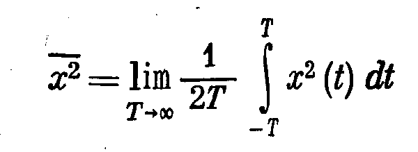
практически
во всех случаях является наиболее просто
вычисляемой величиной, что и определило
использование этого критерия.

Возможны
несколько формулировок задачи. Наиболее
просто задача может быть сформулирована
так. Если имеется какая-то система
автоматического регулирования
заданной структуры, то необходимо так
выбрать параметры этой системы, чтобы
получить минимум среднеквадратичной
ошибки при заданных статистических
характеристиках полезного сигнала и
помехи.

Эта
задача решается следующим образом. По
спектральной плотности ошибки путем
ее интегрирования находится дисперсия.
Дисперсия получается зависящей от
вероятностных характеристик полезного
сигнала, помехи и параметров системы.
Затем ищутся условия, которые должны
быть наложены на параметры системы,
чтобы получить минимум дисперсии. При
достаточно простом выражении для
дисперсии это может быть определено
непосредственным дифференцированием
и приравниванием нулю частных производных.

В
более сложных случаях приходится искать
минимум дисперсии путем числового
задания интересующих параметров и
построения соответствующих графиков,
а также расчетом на ЭВМ.

Нахождение
оптимальной передаточной функции еще
не означает, что реальная автоматическая
система может быть выполнена оптимальной,
так как реализация ее может быть сопряжена
с большими трудностями. Оптимальную
передаточную функцию, за исключением
простейших случаев, следует считать
идеальной функцией, к которой по
возможности надо стремиться при
выполнении реальной автоматической
системы.

Вопросы
самоконтроля:

Какую
величину используют для оценки точности
автоматической системы со случайными
сигналами.
Дайте
определение критерию
минимума среднеквадратичной ошибки
при одновременном действии полезного
сигнала и помехи.
Как
определяется минимум
дисперсии.

Соседние файлы в папке лекции

Критерий — минимум — среднеквадратичная ошибка

Cтраница 1

Критерий минимума среднеквадратичной ошибки используется для решения более сложных задач по сравнению с задачей определения оптимальных параметров при известной структуре системы.
[1]

Идея приближения по критерию минимума среднеквадратичной ошибки, как уже указывалось, не единственна.
[2]

Тх корректирующего устройства по критерию минимума среднеквадратичной ошибки, если полезный сигнал и помеха независимы и приложены к одной точке системы.
[3]

Первое из этих условий удовлетворялось и при синтезе по критерию минимума среднеквадратичной ошибки.
[4]

Адекватность полученной модели и необходимость ее коррекции оценивают чаще всего по критерию минимума среднеквадратичной ошибки. Этот метод наиболее целесообразен.
[5]

Причем объем вычислений может быть значительно уменьшен за счет незначительного ухудшения качества, фильтрации по критерию минимума среднеквадратичной ошибки.
[6]

В большинстве практически встречающихся случаев представляется возможным, хотя бы в первом приближении, рассматривать процессы изменения технологических величин или других производственных показателей как стационарные случайные функции с нормальным распределением. Поэтому обычно критерий минимума среднеквадратичной ошибки является наиболее приемлемым в качестве критерия наилучшего предсказания в большинстве рассматриваемых задач управления.
[7]

Кроме того, по критерию минимума среднеквадратичной ошибки определяются оптимальная структура и передаточная функция замкнутой системы, обеспечивающие минимальную величину погрешности.
[8]

Анализ и синтез нелинейных систем с неизвестной структурой предлагается проводить с помощью многопеременных прямоугольных функций. Практически реализуемый алгоритм с применением этих функций получен на основе критерия минимума среднеквадратичной ошибки. Алгоритм применим при входных стационарных сигналах с произвольной плотностью распределения вероятностей.
[9]

Задача заключается в оценке значений, к-рые реализация рассматриваемого процесса ( или нек-рых его параметров, таких, как ср. Здесь в большинстве случаев определяется инвариантный во времени линейный реализуемый фильтр, оптимизирующий оценку по критерию минимума среднеквадратичной ошибки. Возможны и часто желательны др. критерии, но указанный критерий отличается математич. Для решения задач такого рода часто применяется теория Винера — Колмогорова. В этой теории предполагается, что сигнал S ( t) характеризуется только статистич. Мешающий шум N ( t) представляет также чисто случайный процесс, комбинируется с сигналом аддитивно и может быть с ним связан статистически. Далее предполагается, что накопление и обработка данных совершаются только над прошлым процессов на входе, к-рые считаются стационарными в широком смысле и имеющими положительно определенные ковариант-ные ф-ции. Кроме того, в большинстве случаев реализуются оптимальные линейные фильтры, к-рые не только реализуемы, но также и инвариантны во времени. При этих условиях импульсная переходная ф-ция линейного фильтра определяется из интегр.
[10]

Задача заключается в оценке значений, к-рые реализация рассматриваемого процесса ( или нек-рых его параметров, таких, как ср. Здесь в большинство случаев определяется инвариантный во времени линейный реализуемый фильтр, оптимизирующий оценку по критерию минимума среднеквадратичной ошибки. Возможны и часто желательны др. критерии, но указанный критерий отличается математич. Для решения задач такого рода часто применяется теория Винера — Колмогорова. В этой теории предполагается, что сигнал S ( t) характеризуется только статпстич. Мешающий шум N ( t) представляет также чисто случайный процесс, комбинируется с сигналом аддитивно и может быть с ним связан статистически. Далее предполагается, что накопление и обработка данных совершаются только над прошлым процессов па входе, к-рые считаются стационарными в широком смысле и имеющими положительно определенные ковариант-ные ф-ции. Кроме того, в большинстве случаев реализуются оптимальные линейные фильтры, к-рые не только реализуемы, но также и инвариантны во времени. При этих условиях импульсная переходная ф-ция линейного фильтра определяется из интегр.
[11]

После определения среднеквадратичной ошибки необходимо обеспечить минимальное значение ее. Наиболее просто задача решается путем минимизации среднеквадратичной ошибки по тому или иному параметру системы при заданных воздействиях. В качестве параметров, которые желательно сделать оптимальными на основе критерия минимума среднеквадратичной ошибки, могут рассматриваться различные постоянные, имеющие большое значение для определения динамических свойств системы.
[12]

Страницы:

Анализ систем на основе критерия минимума среднеквадратичной ошибки [c.189]

Если ковариационные функции процессов Х( ) и У(/) известны точно, то можно воспользоваться винеровским критерием минимума среднеквадратичной ошибки Этот критерий утверждает, что функция /г(и) должна быть выбрана так, чтобы минимизировать среднеквадратичную ошибку шумовой компоненты, т е [c.190]

Синтез следящих систем. Одно из первых инженерных применений анализа на основе критерия минимума среднеквадратичной ошибки было сделано при синтезировании следящих систем для зенитных орудий и в радиолокационных следящих системах [5] Например, от радиолокационной следящей системы требуется, чтобы она следила за самолетом несмотря на возмущения отра- [c.189]

Другое применение критерий минимума среднеквадратичной ошибки находит в задаче об идентификации системы В этом случае в распоряжении имеются входной сигнал и соответствующий ему выходной сигнал от некоторой системы, требуется вывести линейное приближение к этой системе для дальнейшего его использования при управлении или моделировании Предположим, например, что система представляет собой черный ящик (рис 5 7). Если вход является реализацией случайного процесса Х 1), то выход можно рассматривать как реализацию случайного процесса У(0< где [c.190]

Оптимальное в любом смысле корреляционное окно, например (7 2 3), будет зависеть от неизвестного спектра Гхх(/). Этот недостаток свойствен не только спектральному анализу Вообще говоря, справедливо правило, согласно которому наилучший план действий должен опираться на некоторые представления об истинном положении вещей Следовательно, очень валено проводить четкое различие между планированием спектрального анализа до сбора данных и самим анализом данных, после того как они собраны Мы хотели бы использовать критерии минимума среднеквадратичной ошибки или какой-нибудь аналогичный критерий до проведения спектрального анализа, чтобы решить, например, какой длины нужно взять запись Но после того как данные собраны, могло бы оказаться, что наши представления относительно Гхх (/) были абсолютно неправильны [c.26]

Если плотность вероятности ге ([х у) симметрична относительно среднего значения гпг [х у и унимодальна (т. е. монотонно невозрастающая функция [х — /П] [х у ), то байесовская оценка (5.18) совпадает с оценкой по критерию максимума апостериорной плотности вероятности. В этом случае функция С (х) не должна быть обязательно выпуклой, а лишь монотонно неубывающей функцией х (см. приложение С). Так как нормальная плотность вероятности унимодальна, то всегда, когда плотность вероятности ге ([х I у) нормальна, оценка по максимуму апостериорной плотности вероятности совпадает с широким классом байесовских оценок, который включает оценки по минимуму среднеквадратичной ошибки (или минимуму дисперсии). [c.158]

Источник

Среднеквадратичная ошибка (Mean Squared Error) – Среднее арифметическое (Mean) квадратов разностей между предсказанными и реальными значениями Модели (Model) Машинного обучения (ML):

MSE как среднее дистанций между предсказаниями и реальными наблюдениями

Рассчитывается с помощью формулы, которая будет пояснена в примере ниже:

$$MSE = frac{1}{n} × sum_{i=1}^n (y_i — widetilde{y}_i)^2$$
$$MSEspace{}{–}space{Среднеквадратическая}space{ошибка,}$$
$$nspace{}{–}space{количество}space{наблюдений,}$$
$$y_ispace{}{–}space{фактическая}space{координата}space{наблюдения,}$$
$$widetilde{y}_ispace{}{–}space{предсказанная}space{координата}space{наблюдения,}$$

MSE практически никогда не равен нулю, и происходит это из-за элемента случайности в данных или неучитывания Оценочной функцией (Estimator) всех факторов, которые могли бы улучшить предсказательную способность.

Пример. Исследуем линейную регрессию, изображенную на графике выше, и установим величину среднеквадратической Ошибки (Error). Фактические координаты точек-Наблюдений (Observation) выглядят следующим образом:

Мы имеем дело с Линейной регрессией (Linear Regression), потому уравнение, предсказывающее положение записей, можно представить с помощью формулы:

$$y = M * x + b$$
$$yspace{–}space{значение}space{координаты}space{оси}space{y,}$$
$$Mspace{–}space{уклон}space{прямой}$$
$$xspace{–}space{значение}space{координаты}space{оси}space{x,}$$
$$bspace{–}space{смещение}space{прямой}space{относительно}space{начала}space{координат}$$

Параметры M и b уравнения нам, к счастью, известны в данном обучающем примере, и потому уравнение выглядит следующим образом:

$$y = 0,5252 * x + 17,306$$

Зная координаты реальных записей и уравнение линейной регрессии, мы можем восстановить полные координаты предсказанных наблюдений, обозначенных серыми точками на графике выше. Простой подстановкой значения координаты x в уравнение мы рассчитаем значение координаты ỹ:

Рассчитаем квадрат разницы между Y и Ỹ:

Сумма таких квадратов равна 4 445. Осталось только разделить это число на количество наблюдений (9):

$$MSE = frac{1}{9} × 4445 = 493$$

Само по себе число в такой ситуации становится показательным, когда Дата-сайентист (Data Scientist) предпринимает попытки улучшить предсказательную способность модели и сравнивает MSE каждой итерации, выбирая такое уравнение, что сгенерирует наименьшую погрешность в предсказаниях.

MSE и Scikit-learn

Среднеквадратическую ошибку можно вычислить с помощью SkLearn. Для начала импортируем функцию:

import sklearn
from sklearn.metrics import mean_squared_error

Инициализируем крошечные списки, содержащие реальные и предсказанные координаты y:

y_true = [5, 41, 70, 77, 134, 68, 138, 101, 131]
y_pred = [23, 35, 55, 90, 93, 103, 118, 121, 129]

Инициируем функцию mean_squared_error(), которая рассчитает MSE тем же способом, что и формула выше:

mean_squared_error(y_true, y_pred)

Интересно, что конечный результат на 3 отличается от расчетов с помощью Apple Numbers:

496.0

Ноутбук, не требующий дополнительной настройки на момент написания статьи, можно скачать здесь.

Автор оригинальной статьи: @mmoshikoo

Фото: @tobyelliott

Источник

Существует идеальная аналогия между векторами и сигналами.

Вектор

Вектор содержит величину и направление. Название вектора обозначается жирным шрифтом, а его величина – светлым.

Пример: V – вектор с величиной V. Рассмотрим два вектора V ₁ и V _2, как показано на следующей диаграмме. Пусть составляющая V ₁ наряду с V ₂ задается C ₁₂ V ₂ . Компонент вектора V ₁ вместе с вектором V ₂ можно получить, взяв перпендикуляр от конца V ₁ к вектору V _2, как показано на диаграмме:

Вектор V ₁ можно выразить через вектор V _2.

V ₁ = C ₁₂ V ₂ + V _e

Где Ve – вектор ошибки.

V ₁ = C ₁₂ V ₂ + V _e

Где Ve – вектор ошибки.

Но это не единственный способ выразить вектор V ₁ через V ₂ . Альтернативные возможности:

V ₁ = C ₁ V ₂ + V _e1

V ₂ = C ₂ V ₂ + V _e2

Сигнал ошибки является минимальным для большого значения компонента. Если C ₁₂ = 0, то два сигнала называются ортогональными.

Точечный продукт двух векторов

V ₁ . V ₂ = V ₁ .V ₂ cosθ

θ = угол между V1 и V2

V ₁ . V ₂ = V ₂ .V ₁

Компоненты V ₁ alog _n V ₂ = V ₁ Cos θ = V1.V2 overV2

V ₁ . V ₂ = V ₁ .V ₂ cosθ

θ = угол между V1 и V2

V ₁ . V ₂ = V ₂ .V ₁

Компоненты V ₁ alog _n V ₂ = V ₁ Cos θ = V1.V2 overV2

Из диаграммы составляющие V ₁ alog _n V ₂ = C ₁₂ V ₂

V1.V2 overV2=C12V2

RightarrowC12=V1.V2 overV2

Сигнал

Понятие ортогональности может быть применено к сигналам. Рассмотрим два сигнала f ₁ (t) и f ₂ (t). Подобно векторам, вы можете аппроксимировать f ₁ (t) в терминах f ₂ (t) как

f ₁ (t) = C ₁₂ f ₂ (t) + f _e (t) для (t ₁ <t <t ₂ )

Rightarrow f _e (t) = f ₁ (t) – C ₁₂ f ₂ (t)

f ₁ (t) = C ₁₂ f ₂ (t) + f _e (t) для (t ₁ <t <t ₂ )

Rightarrow f _e (t) = f ₁ (t) – C ₁₂ f ₂ (t)

Одним из возможных способов минимизации ошибки является интегрирование в интервале от t ₁ до t ₂ .

1 overt2−t1 intt2t1[fe(t)]dt

1 overt2−t1 intt2t1[f1(t)−C12f2(t)]dt

Однако этот шаг также не уменьшает ошибку в значительной степени. Это можно исправить, взяв квадрат функции ошибки.

varepsilon=1 overt2−t1 intt2t1[fe(t)]2dt

Rightarrow1 overt2−t1 intt2t1[fe(t)−C12f2]2dt

Где ε – среднеквадратичное значение сигнала ошибки. Значение C _12, которое минимизирует ошибку, необходимо рассчитать d varepsilon overdC12=0

Rightarrowd overdC12[1 overt2−t1 intt2t1[f1(t)−C12f2(t)]2dt]=0

Rightarrow1 overt2−t1 intt2t1[d overdC12f21(t)−d overdC122f1(t)C12f2(t)+d overdC12f22(t)C212]dt=0

Производные от терминов, которые не имеют C12, равны нулю.

Rightarrow intt2t1−2f1(t)f2(t)dt+2C12 intt2t1[f22(t)]dt=0

Если C12= intt2t1f1(t)f2(t)dt over intt2t1f22(t)dt компонент равен нулю, тогда два сигнала называются ортогональными.

Положите C ₁₂ = 0, чтобы получить условие ортогональности.

0 = intt2t1f1(t)f2(t)dt over intt2t1f22(t)dt

intt2t1f1(t)f2(t)dt=0

Ортогональное векторное пространство

Полный набор ортогональных векторов называется ортогональным векторным пространством. Рассмотрим трехмерное векторное пространство, как показано ниже:

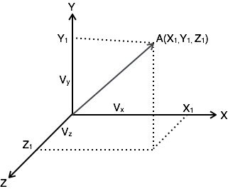
Рассмотрим вектор A в точке (X ₁ , Y ₁ , Z ₁ ). Рассмотрим три единичных вектора (V _X , V _Y , V _Z ) в направлении оси X, Y, Z соответственно. Поскольку эти единичные векторы взаимно ортогональны, он удовлетворяет

$$ V_X. V_X = V_Y. V_Y = V_Z. V_Z = 1 $$

$$ V_X. V_Y = V_Y. V_Z = V_Z. V_X = 0 $$

Вы можете написать выше условия как

$$ V_a. V_b = left { begin {array} {ll} 1 & quad a = b \ 0 & quad a neq b end {array} right. $$

Вектор A может быть представлен в терминах его компонентов и единичных векторов как

A=X1VX+Y1VY+Z1VZ................(1)

Любые векторы в этом трехмерном пространстве могут быть представлены только через эти три единичных вектора.

Если вы рассматриваете n-мерное пространство, то любой вектор A в этом пространстве можно представить как

A=X1VX+Y1VY+Z1VZ+...+N1VN.....(2)

Поскольку величина единичных векторов равна единице для любого вектора A

Компонент А вдоль оси х = AV _X

Компонента А вдоль оси Y = AV _Y

Компонента А вдоль оси Z = AV _Z

Аналогично, для n-мерного пространства компонента A вдоль некоторой оси G

=A.VG...............(3)

Подставьте уравнение 2 в уравнение 3.

RightarrowCG=(X1VX+Y1VY+Z1VZ+...+G1VG...+N1VN)VG

= X_1 V_X V_G + Y_1 V_Y V_G + Z_1 V_Z V_G + … + G_1V_G V_G … + N_1V_N V_G

= G_1 , , , , , text {since} V_G V_G = 1

If V_G V_G neq 1 , , text {т.е.} V_G V_G = k

AV_G = G_1V_G V_G = G_1K

G_1 = {(AV_G) over K}

Ортогональное пространство сигнала

Рассмотрим набор из n взаимно ортогональных функций x ₁ (t), x ₂ (t) … x _n (t) на интервале от t ₁ до t ₂ . Поскольку эти функции ортогональны друг другу, любые два сигнала x _j (t), x _k (t) должны удовлетворять условию ортогональности. т.е.

int_ {t_1} ^ {t_2} x_j (t) x_k (t) dt = 0 , , , text {where} , j neq k

text {Let} int_ {t_1} ^ {t_2} x_ {k} ^ {2} (t) dt = k_k

Пусть функция f (t) может быть аппроксимирована этим пространством ортогональных сигналов путем сложения компонентов вдоль взаимно ортогональных сигналов, т.е.

, , , f (t) = C_1x_1 (t) + C_2x_2 (t) + … + C_nx_n (t) + f_e (t)

quad quad = Sigma_ {r = 1} ^ {n} C_rx_r (t)

, , , f (t) = f (t) – Sigma_ {r = 1} ^ n C_rx_r (t)

, , , f (t) = C_1x_1 (t) + C_2x_2 (t) + … + C_nx_n (t) + f_e (t)

quad quad = Sigma_ {r = 1} ^ {n} C_rx_r (t)

, , , f (t) = f (t) – Sigma_ {r = 1} ^ n C_rx_r (t)

Средняя квадратура ошибки varepsilon = {1 over t_2 – t_2} int_ {t_1} ^ {t_2} [f_e (t)] ^ 2 dt

= {1 over t_2 – t_2} int_ {t_1} ^ {t_2} [f [t] – sum_ {r = 1} ^ {n} C_rx_r (t)] ^ 2 dt

Компонент, который минимизирует среднеквадратичную ошибку, может быть найден

{d varepsilon over dC_1} = {d varepsilon over dC_2} = … = {d varepsilon over dC_k} = 0

Рассмотрим {d varepsilon over dC_k} = 0

{d over dC_k} [{1 over t_2 – t_1} int_ {t_1} ^ {t_2} [f (t) – Sigma_ {r = 1} ^ n C_rx_r (t)] ^ 2 dt] = 0

Все члены, которые не содержат C _k , равны нулю. т.е. в сумме, r = k терм остается, а все остальные термы равны нулю.

int_ {t_1} ^ {t_2} – 2 f (t) x_k (t) dt + 2C_k int_ {t_1} ^ {t_2} [x_k ^ 2 (t)] dt = 0

Rightarrow C_k = {{ int_ {t_1} ^ {t_2} f (t) x_k (t) dt} over {int_ {t_1} ^ {t_2} x_k ^ 2 (t) dt}}

Rightarrow int_ {t_1} ^ {t_2} f (t) x_k (t) dt = C_kK_k

Средняя квадратическая ошибка

Среднее квадрата ошибки функция f _e (t) называется среднеквадратичной ошибкой. Обозначается через ε (эпсилон).

varepsilon = {1 over t_2 – t_1} int_ {t_1} ^ {t_2} [f_e (t)] ^ 2dt

, , , , = {1 over t_2 – t_1} int_ {t_1} ^ {t_2} [f_e (t) – Sigma_ {r = 1} ^ n C_rx_r (t)] ^ 2 дт

, , , , = {1 over t_2 – t_1} [ int_ {t_1} ^ {t_2} [f_e ^ 2 (t)] dt + Sigma_ {r = 1} ^ {n} C_r ^ 2 int_ {t_1} ^ {t_2} x_r ^ 2 (t) dt – 2 Sigma_ {r = 1} ^ {n} C_r int_ {t_1} ^ {t_2} x_r (t) f (t) dt

Вы знаете, что C_ {r} ^ {2} int_ {t_1} ^ {t_2} x_r ^ 2 (t) dt = C_r int_ {t_1} ^ {t_2} x_r (t) f (d) dt = C_r ^ 2 К_р

varepsilon = {1 over t_2 – t_1} [ int_ {t_1} ^ {t_2} [f ^ 2 (t)] dt + Sigma_ {r = 1} ^ {n} C_r ^ 2 K_r – 2 Sigma_ {r = 1} ^ {n} C_r ^ 2 K_r]

, , , , = {1 over t_2 – t_1} [ int_ {t_1} ^ {t_2} [f ^ 2 (t)] dt – Sigma_ {r = 1} ^ {n} C_r ^ 2 K_r]

, следовательно varepsilon = {1 over t_2 – t_1} [ int_ {t_1} ^ {t_2} [f ^ 2 (t)] dt + (C_1 ^ 2 K_1 + C_2 ^ 2 K_2 + … + C_n ^ 2 K_n)]

Приведенное выше уравнение используется для оценки среднеквадратичной ошибки.

Закрытый и полный набор ортогональных функций

Рассмотрим набор из n взаимно ортогональных функций x ₁ (t), x ₂ (t) … x _n (t) на интервале от t ₁ до t ₂ . Это называется замкнутым и полным набором, когда не существует функции f (t), удовлетворяющей условию int_ {t_1} ^ {t_2} f (t) x_k (t) dt = 0

Если эта функция удовлетворяет уравнению int_ {t_1} ^ {t_2} f (t) x_k (t) dt = 0 , , text {for} , k = 1,2, .. , то f (t) называется ортогональным к каждой функции ортогонального множества. Это множество неполное без f (t). Это становится закрытым и полным набором, когда f (t) включен.

f (t) может быть аппроксимирован этим ортогональным набором путем сложения компонентов вдоль взаимно ортогональных сигналов, т.е.

f (t) = C_1 x_1 (t) + C_2 x_2 (t) + … + C_n x_n (t) + f_e (t)

Если бесконечный ряд C_1 x_1 (t) + C_2 x_2 (t) + … + C_n x_n (t) сходится к f (t), то среднеквадратичная ошибка равна нулю.

Ортогональность в сложных функциях

Если f ₁ (t) и f ₂ (t) являются двумя комплексными функциями, то f ₁ (t) можно выразить через f ₂ (t) как

f_1 (t) = C_ {12} f_2 (t) , , , , , , , , ..с незначительной ошибкой

Где C_ {12} = {{ int_ {t_1} ^ {t_2} f_1 (t) f_2 ^ * (t) dt} over { int_ {t_1} ^ {t_2} | f_2 (t) | ^ 2 dt}}

Где f_2 ^ * (t) = комплексное сопряжение f ₂ (t).

Если f ₁ (t) и f ₂ (t) ортогональны, то C ₁₂ = 0

{ int_ {t_1} ^ {t_2} f_1 (t) f_2 ^ * (t) dt over int_ {t_1} ^ {t_2} | f_2 (t) | ^ 2 dt} = 0

Rightarrow int_ {t_1} ^ {t_2} f_1 (t) f_2 ^ * (dt) = 0

Приведенное выше уравнение представляет условие ортогональности в комплексных функциях.

Источник

On Nonidentical Discrete-Time Hyperchaotic Systems Synchronization: Towards Secure Medical Image Transmission

3.3 Measurement of Encryption and Decryption Quality

Multichannel Image Recovery

3.1 Linear Minimum Mean Square Error (LMMSE) Estimation

Regression analysis

3 Cost functions

3.1 MSE

3.2 MSLE

3.3 RMSE

3.4 MAE

Optimization of Methods for Image-Texture Segmentation Using Ant Colony Optimization

2.4 Evaluation of Segmentation Techniques

2.4.1 Mean-Square Error

2.4.2 Root-Mean-Square-Error

2.4.3 Signal-to-Noise Ratio

2.4.4 Peak Signal-to-Noise Ratio

Uplink Physical Layer Functions

10.9.5.1 LMMSE receiver

Digital Picture Formats and Representations

Peak signal to noise ratio (PSNR)

Energy-Efficient MIMO–OFDM Systems

15.2.1.2.2 MMSE Detection Algorithm

Mean-Square Error Linear Estimation

4.1 Introduction

Accruement of nonlinear dynamical system and its dynamics: electronics and cryptographic engineering

Mean square error (MSE)

Detection methods

6.3.3 Complexity

Мотивация

Определение

Характеристики

Линейный оценщик MMSE

Одномерный случай

Вычисление

Линейная оценка MMSE для процесса линейного наблюдения

Альтернативная форма

Последовательная линейная оценка MMSE

Частный случай: скалярные наблюдения

Примеры

Пример 1

Пример 2

Пример 3

Пример 4

Смотрите также

Примечания

дальнейшее чтение

Motivation[edit]

Definition[edit]

Properties[edit]

Linear MMSE estimator[edit]

Univariate case[edit]

Computation[edit]

Linear MMSE estimator for linear observation process[edit]

Alternative form[edit]

Sequential linear MMSE estimation[edit]

Special case: scalar observations[edit]

Examples[edit]

Example 1[edit]

Example 2[edit]

Example 3[edit]

Example 4[edit]

See also[edit]

Notes[edit]

Further reading[edit]

Motivation[edit]

Definition[edit]

Properties[edit]

Linear MMSE estimator[edit]

Univariate case[edit]

Computation[edit]

Linear MMSE estimator for linear observation process[edit]

Alternative form[edit]

Sequential linear MMSE estimation[edit]

Special case: scalar observations[edit]

Examples[edit]

Example 1[edit]

Example 2[edit]

Example 3[edit]

Example 4[edit]

See also[edit]