Средняя квадратическая ошибка положения

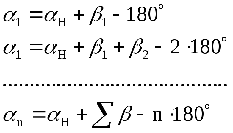
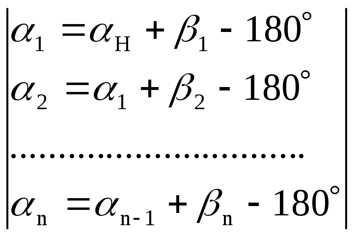
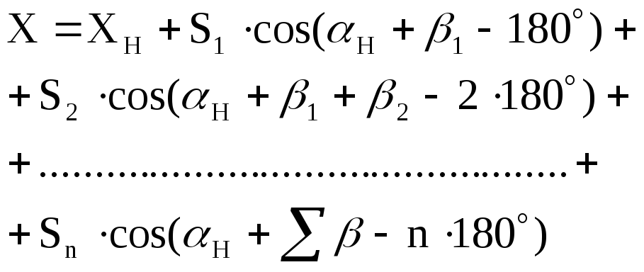
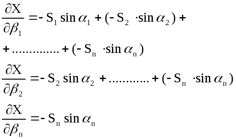
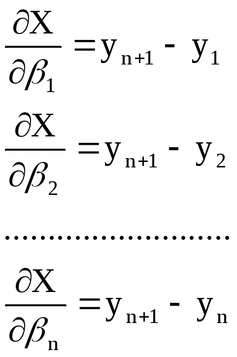
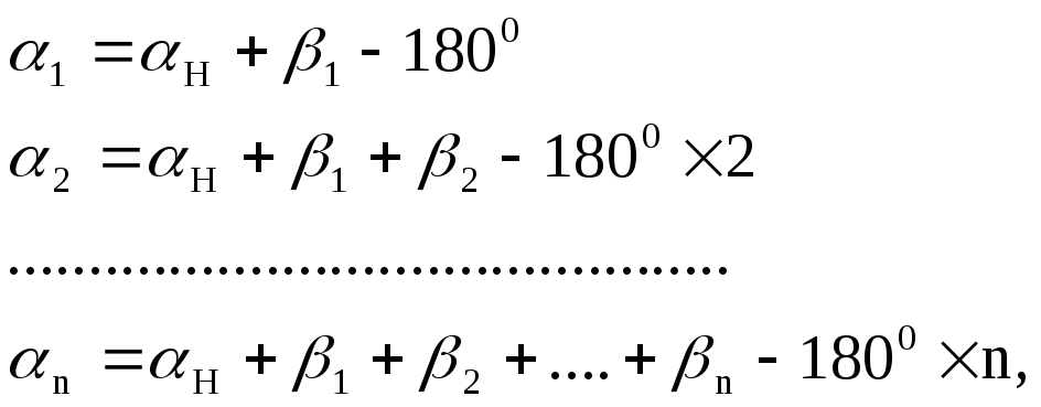
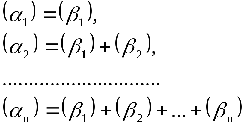
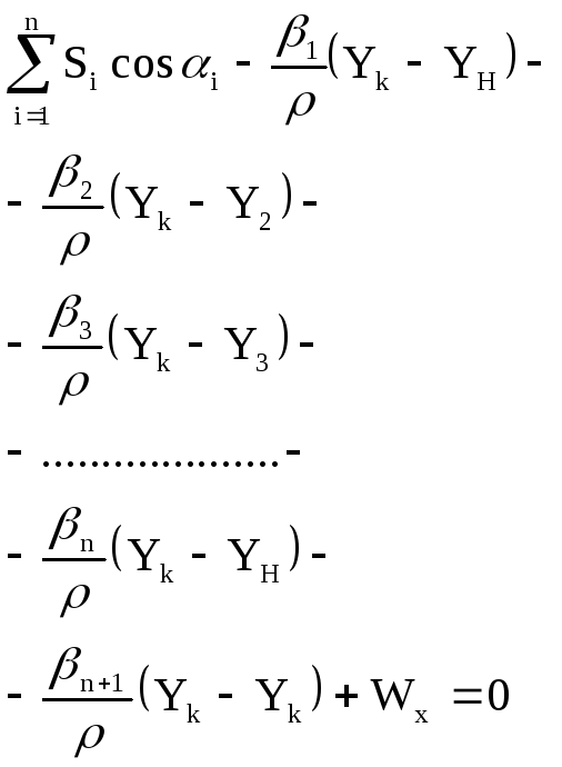
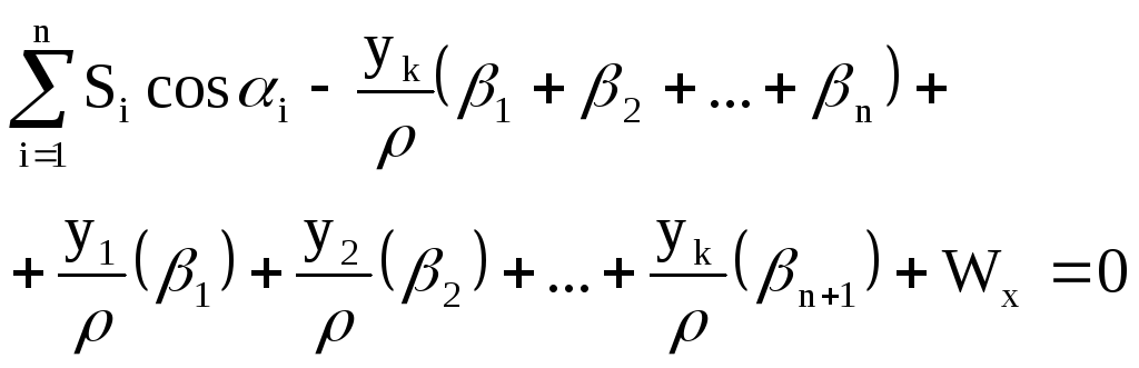
Выразим α через
β:

.

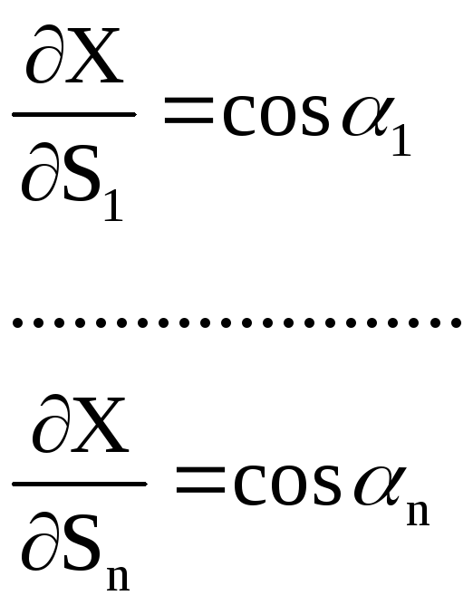
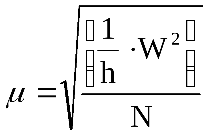
5.Оценка точности угловых измерений по невязкам полигонах

1. по
   сумме углов:

;

,

где
N–
число невязок.

1. сумме
   превышений:

,

где
L–
длина хода, км.

1. по
   разностям двойных измерений:

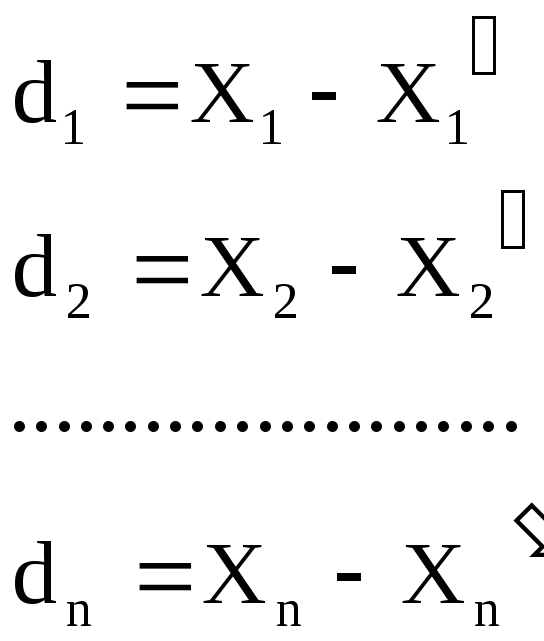
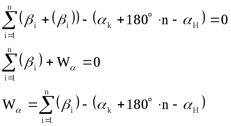
6. Условные уравнения в полигонометрическом ходе

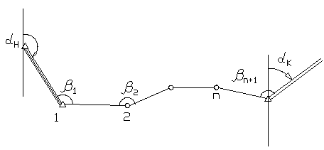
1)условное уравнение
дирекционных углов:

1. условные
   уравнения координат:

Выразим
эти условные уравнения через поправки.
Для этого первое из них запишем в виде

(1)

Выводы для второго
уравнения аналогичны, поэтому они не
приводятся.

Разлагая
условное уравнение координат в ряд
Тейлора по поправкам, получим:

,
(2)

где

(3) Поправки
в дирекционные углы выразим через
поправки в измеренные углы. Поскольку

то

Подставляем эти
значения в условные уравнения (2):

.

Многомерный статистический анализ

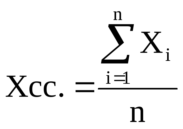
1. Среднее
   значение и корреляционная матрица
   вектора

Если задана функция:

,

то

Нормальное
распределение

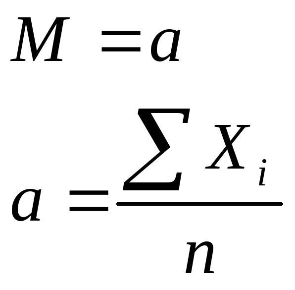
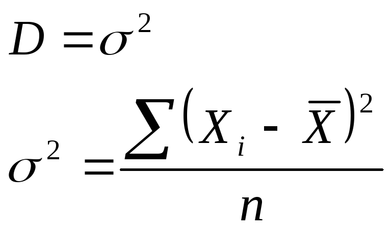
1. одномерное
   распределение. Математическое ожидание(М)
   и дисперсия(D)

Одномерное
распределение – это такое распределение,
где исследуется один признак.

Функция нормального
распределения:

,

где
–
стандарт;

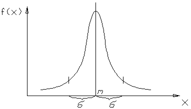
Свойства
функции: 1)всякая кривая достигает точки
максимума в точке X=m;

2)функция
непрерывна и приближается к оси Х;

3)симметрична
относительно прямой, параллельной f(х),
максимальная ордината –
;

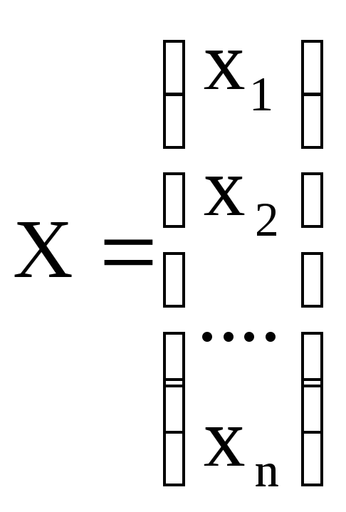
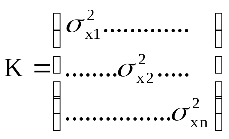
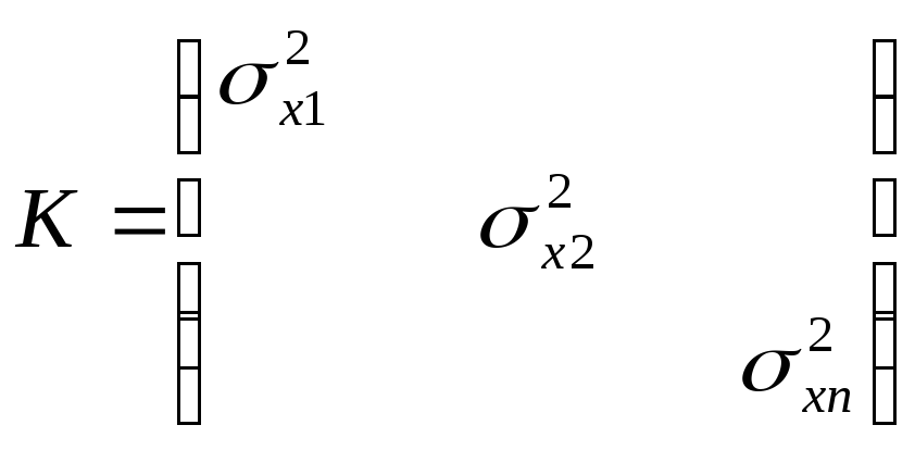
2.Многомерное
нормальное распределение

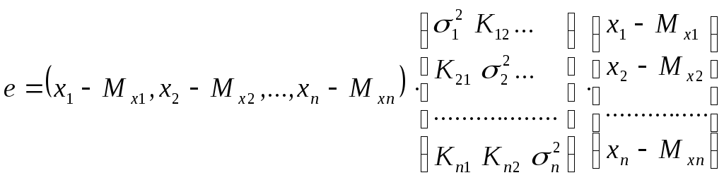
Многомерное
нормальное распределение – распределение,
характеризующееся вектором случайных
величин, заданным математическим
ожиданием этого вектора и корреляционной
матрицей.

; ;

.

V–
отклонение вектора, от его математического
ожидания (Х_n-М_хn)

Метод наименьших
квадратов

1.Параметрический
способ уравнивания

Одну
и ту же функцию можно выразить как через
вектор параметров (Х), так и через вектор
измерений (L)

Задача
уравнивания сводиться к получению
достаточной, несмещенной и эффективной
оценке функции Z.

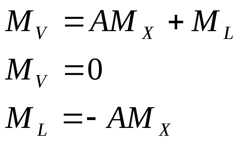
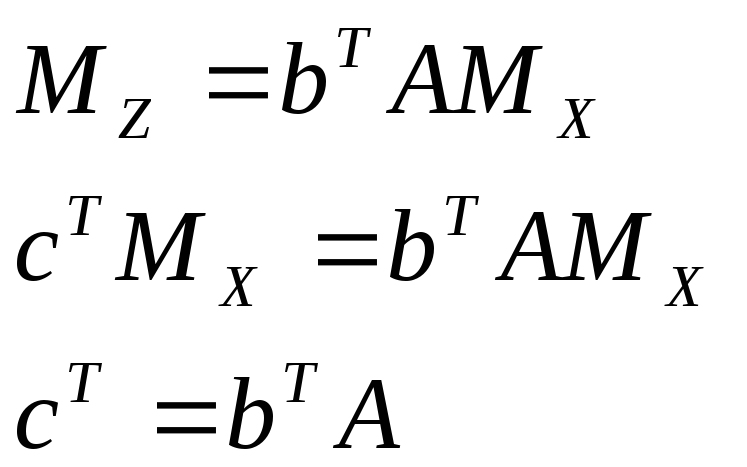
А) для получения
несмещенной оценки запишем математическое
ожидание:

Составляем систему
уравнений поправок:

.

(1)

Это и есть условие
несмещенности.

В)
чтобы оценка была эффективной, дисперсия
функции Z
должна быть минимальной.

Найдем минимум
функционала Лагранжа:

,

где Λ– вектор
неопределенного множителя Лагранжа.

Найдем производную
по вектору b и приравняем ее к нулю:

(2)

Вектор
множителя Λ – неизвестен.

Подставляем (2) в
(1):

(3)

Далее, (3) подставляем
в (2):

.

При
таком значении b получается достаточная,
несмещенная и эффективная оценка функции
Z.

Частный
случай:

если

,

где
Е– единичная матрица,то

1. Коррелатный способ уравнивания

После уравнивания
геодезической сети, любая функция
уравненных величин, должна определяться
однозначно при любом порядке ее
вычисления.

Получаемые
после уравнивания оценки любых функций
уравненных результатов измерений должны
быть достаточными, несмещенными и
эффективными.

Введем обозначения:

F(y)–
функция результатов измерений;

у – вектор
результатов измерений;

у=Y+Δ,

где
Y–
вектор истинных значений измеренных
величин;

Δ – вектор истинных
ошибок.

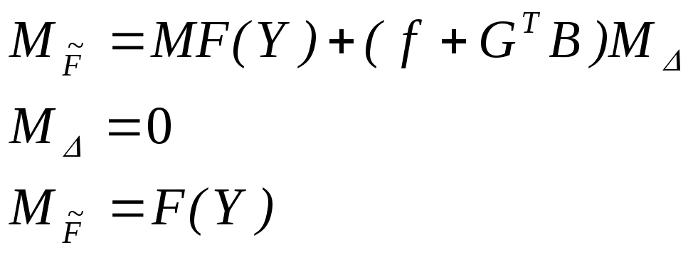
Линеаризированный
вид функции:

1. С
   тем, чтобы оценка была достаточной,
   необходимо ее выводить с учетом всех
   измерений в геодезической сети

,

где
W
– вектор свободных членов;

G
– матрица, которую следует определить.

2)
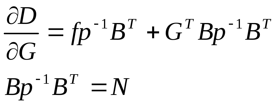
Для достижения эффективности оценки
следует найти такую матрицу G,
при которой достигается минимальная
дисперсия

F(Y)–
безошибочна, так как Y–
истинное значение

,

где
В – матрица коэффициентов условных
уравнений

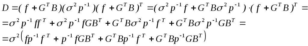
Вид
оцениваемой функции:

,

а
ее дисперсия

,

где

–
корреляционная матрица ошибок.

,

где
–
поправка.

3)Полученное
значение будет несмещенным, если ошибки
измерений случайны:

Соседние файлы в предмете [НЕСОРТИРОВАННОЕ]

• #
• #
• #
• #
• #
• #
• #
• #
• #
• #
• #

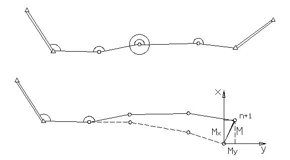
7.4 Средняя квадратическая ошибка положения конечной точки полигонометрии

Ход вытянутый (углы не исправлены за невязку).

Ранее были получены формулы для вычисления компонентов ,  (7.20) и (7.28)

; 

По этим величинам можно найти среднюю квадратическую ошибку самого вектора М (рис.7.4) по формуле:

 (7.29)

а подставив значение из (7.20) и (7.28) получим:

 (7.30)

Эта величина называется средней квадратической ошибкой положения конечной точки хода полигонометрии.

Как видно из (7.30), ошибка последнего угла _n+1 не оказывает влияния на величину поперечной невязки, т.е. ход считается как бы висячим. Это и понятно, т. к. углы за угловую невязку не исправлялись.

На практике углы, как правило, исправляются за угловую невязку путем ее распределения поровну на все углы. В этом случае поперечная невязка будет другая, поэтому будет другая формула для вычисления средней квадратической ошибки положения конечной точки хода полигонометрии. Эта формула приводится в конце этого параграфа.

. Ход изогнутый (углы не исправлены за угловую невязку).

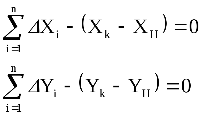
В ходе полигонометрии произвольной формы возникают невязки _x, _y, _S, вычисляемые по формулам (7.17), (7.18).

Если в одном и том же ходе измерить все углы и линии «k» раз, то можно найти «k» значений невязок _x, _y, _S, т.е.

Сложив почленно все равенства и разделив левую и правую части на «k», получим:

Каждый член этого равенства является соответствующим средним квадратическим значением. Поэтому равенство можно переписать

 (7.31)

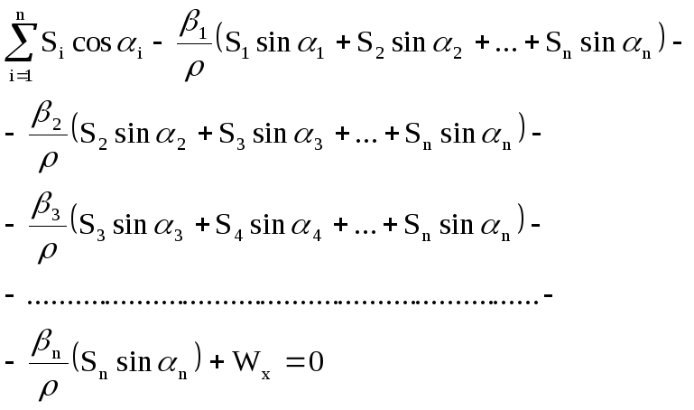
Для установления зависимости между М и ошибками измерения длин линий m_S и углов m_ возьмем без вывода координатные условные уравнения для одиночного хода полигонометрии. (Вывод этих формул будет рассмотрен при изучении уравнивания полигонометрии).

 (7.32)

_i — дирекционный угол линии,

V_S, V_-поправка в измеренные длины и углы,

,  — разности координат конечной и каждой из точек хода,

_x, _y — невязки в приращениях координат, которые являются истинными ошибками в координатах конечного пункта полигонометрии.

Перенеся невязки _x, _y в правую часть будем иметь

 (7.33)

Так как поправка и ошибка различаются между собой только знаком, то можно записать:

, , (7.34)

где dS_i и d_i – ошибки измерения длин линий и углов.

С учетом этого предыдущее выражение (7.33) можно переписать:

 (7.35)

Отсюда по правилам теории ошибок вычисляем средние квадратические ошибки:

 (7.36)

Подставляем эти значения в формулу (7.31), получим среднюю квадратическую ошибку положения конечной точки хода полигонометрии:

,

но так как , то

 (7.37)

Обозначим

 (7.38)

Как видно из рисунка 7.6 D_n+1,i есть расстояние между последней и i‑той точкой хода.

Рисунок 7.6 – Схема для определения средней квадратической ошибки положения конечной точки висячего полигонометрического хода

С учетом (7.38) формулу (7.37) перепишем

 (7.39)

По этой формуле вычисляется средняя квадратическая ошибка положения конечной точки висячего изогнутого полигонометрического хода. По этой же формуле можно вычислить среднюю квадратическую ошибку положения любой точки висячего полигонометрического хода При этом под n подразумевается число линий от начальной точки до определяемой.

Как видно из формулы (7.39) величина М зависит не только от ошибок измерения длин и углов, но и от степени изогнутости хода и количества углов поворота в нем. Величина  тем меньше, чем больше вытянут ход и чем меньше в нем углов поворота.

Полученная формула не учитывает ошибок исходных данных. В этом случае ошибка в положении конечной точки хода будет и невязкой этого хода. В действительности исходные координаты и дирекционные углы сами содержат ошибки, поэтому между невязкой и ошибкой положения точки будет некоторая разница. В этом случае для учета ошибок полевых измерений и ошибок исходных данных пользуются формулой:

 (7.40)

МЕТОДЫ ПРЕДРАСЧЕТА СРЕДНЕЙ КВАДРАТИЧЕСКОЙ ПОГРЕШНОСТИ ПОЛОЖЕНИЯ ПУНКТОВ ПРОЕКТИРУЕМОЙ СЕТИ

Алексенко Анастасия Геннадьевна¹, Гребенщикова Алена Николаевна², Грибунина Ксения Антоновна³, Пучнина Алена Ивановна^4
1Санкт-Петербургский горный университет, кандидат технических наук, ассистент кафедры маркшейдерского дела
²Санкт-Петербургский горный университет, студент кафедры маркшейдерского дела
³Санкт-Петербургский горный университет, студент кафедры маркшейдерского дела
⁴Санкт-Петербургский горный университет, студент кафедры маркшейдерского дела

Аннотация
Статья посвящена сравнению двух способов расчета средней квадратической погрешности положения пунктов сети или хода на этапе их проектирования: расчет по формуле, основанной на законе переноса погрешностей и расчет данной величины в программном продукте Credo_DAT.

Ключевые слова: анализ точности, маркшейдерские измерения, маркшейдерское обеспечение, погрешности измерений, точность измерений

---

Рубрика: 25.00.00 НАУКИ О ЗЕМЛЕ

Библиографическая ссылка на статью:
Алексенко А.Г., Гребенщикова А.Н., Грибунина К.А., Пучнина А.И. Методы предрасчета средней квадратической погрешности положения пунктов проектируемой сети // Современные научные исследования и инновации. 2018. № 5 [Электронный ресурс]. URL: https://web.snauka.ru/issues/2018/05/86604 (дата обращения: 02.06.2023).

From Wikipedia, the free encyclopedia

In statistics, the mean squared error (MSE)^[1] or mean squared deviation (MSD) of an estimator (of a procedure for estimating an unobserved quantity) measures the average of the squares of the errors—that is, the average squared difference between the estimated values and the actual value. MSE is a risk function, corresponding to the expected value of the squared error loss.^[2] The fact that MSE is almost always strictly positive (and not zero) is because of randomness or because the estimator does not account for information that could produce a more accurate estimate.^[3] In machine learning, specifically empirical risk minimization, MSE may refer to the empirical risk (the average loss on an observed data set), as an estimate of the true MSE (the true risk: the average loss on the actual population distribution).

The MSE is a measure of the quality of an estimator. As it is derived from the square of Euclidean distance, it is always a positive value that decreases as the error approaches zero.

The MSE is the second moment (about the origin) of the error, and thus incorporates both the variance of the estimator (how widely spread the estimates are from one data sample to another) and its bias (how far off the average estimated value is from the true value).^{[citation needed]} For an unbiased estimator, the MSE is the variance of the estimator. Like the variance, MSE has the same units of measurement as the square of the quantity being estimated. In an analogy to standard deviation, taking the square root of MSE yields the root-mean-square error or root-mean-square deviation (RMSE or RMSD), which has the same units as the quantity being estimated; for an unbiased estimator, the RMSE is the square root of the variance, known as the standard error.

Definition and basic properties[edit]

The MSE either assesses the quality of a predictor (i.e., a function mapping arbitrary inputs to a sample of values of some random variable), or of an estimator (i.e., a mathematical function mapping a sample of data to an estimate of a parameter of the population from which the data is sampled). The definition of an MSE differs according to whether one is describing a predictor or an estimator.

Predictor[edit]

If a vector of predictions is generated from a sample of data points on all variables, and is the vector of observed values of the variable being predicted, with being the predicted values (e.g. as from a least-squares fit), then the within-sample MSE of the predictor is computed as

In other words, the MSE is the mean of the squares of the errors . This is an easily computable quantity for a particular sample (and hence is sample-dependent).

In matrix notation,

where is and is the column vector.

The MSE can also be computed on q data points that were not used in estimating the model, either because they were held back for this purpose, or because these data have been newly obtained. Within this process, known as statistical learning, the MSE is often called the test MSE,^[4] and is computed as

Estimator[edit]

The MSE of an estimator with respect to an unknown parameter is defined as^[1]

This definition depends on the unknown parameter, but the MSE is a priori a property of an estimator. The MSE could be a function of unknown parameters, in which case any estimator of the MSE based on estimates of these parameters would be a function of the data (and thus a random variable). If the estimator is derived as a sample statistic and is used to estimate some population parameter, then the expectation is with respect to the sampling distribution of the sample statistic.

The MSE can be written as the sum of the variance of the estimator and the squared bias of the estimator, providing a useful way to calculate the MSE and implying that in the case of unbiased estimators, the MSE and variance are equivalent.^[5]

Proof of variance and bias relationship[edit]

An even shorter proof can be achieved using the well-known formula that for a random variable , . By substituting with, , we have

But in real modeling case, MSE could be described as the addition of model variance, model bias, and irreducible uncertainty (see Bias–variance tradeoff). According to the relationship, the MSE of the estimators could be simply used for the efficiency comparison, which includes the information of estimator variance and bias. This is called MSE criterion.

In regression[edit]

In regression analysis, plotting is a more natural way to view the overall trend of the whole data. The mean of the distance from each point to the predicted regression model can be calculated, and shown as the mean squared error. The squaring is critical to reduce the complexity with negative signs. To minimize MSE, the model could be more accurate, which would mean the model is closer to actual data. One example of a linear regression using this method is the least squares method—which evaluates appropriateness of linear regression model to model bivariate dataset,^[6] but whose limitation is related to known distribution of the data.

The term mean squared error is sometimes used to refer to the unbiased estimate of error variance: the residual sum of squares divided by the number of degrees of freedom. This definition for a known, computed quantity differs from the above definition for the computed MSE of a predictor, in that a different denominator is used. The denominator is the sample size reduced by the number of model parameters estimated from the same data, (n−p) for p regressors or (n−p−1) if an intercept is used (see errors and residuals in statistics for more details).^[7] Although the MSE (as defined in this article) is not an unbiased estimator of the error variance, it is consistent, given the consistency of the predictor.

In regression analysis, «mean squared error», often referred to as mean squared prediction error or «out-of-sample mean squared error», can also refer to the mean value of the squared deviations of the predictions from the true values, over an out-of-sample test space, generated by a model estimated over a particular sample space. This also is a known, computed quantity, and it varies by sample and by out-of-sample test space.

Examples[edit]

Mean[edit]

Suppose we have a random sample of size from a population, . Suppose the sample units were chosen with replacement. That is, the units are selected one at a time, and previously selected units are still eligible for selection for all draws. The usual estimator for the is the sample average

which has an expected value equal to the true mean (so it is unbiased) and a mean squared error of

where is the population variance.

For a Gaussian distribution, this is the best unbiased estimator (i.e., one with the lowest MSE among all unbiased estimators), but not, say, for a uniform distribution.

Variance[edit]

The usual estimator for the variance is the corrected sample variance:

This is unbiased (its expected value is ), hence also called the unbiased sample variance, and its MSE is^[8]

where is the fourth central moment of the distribution or population, and is the excess kurtosis.

However, one can use other estimators for which are proportional to , and an appropriate choice can always give a lower mean squared error. If we define

then we calculate:

This is minimized when

For a Gaussian distribution, where , this means that the MSE is minimized when dividing the sum by . The minimum excess kurtosis is ,^[a] which is achieved by a Bernoulli distribution with p = 1/2 (a coin flip), and the MSE is minimized for Hence regardless of the kurtosis, we get a «better» estimate (in the sense of having a lower MSE) by scaling down the unbiased estimator a little bit; this is a simple example of a shrinkage estimator: one «shrinks» the estimator towards zero (scales down the unbiased estimator).

Further, while the corrected sample variance is the best unbiased estimator (minimum mean squared error among unbiased estimators) of variance for Gaussian distributions, if the distribution is not Gaussian, then even among unbiased estimators, the best unbiased estimator of the variance may not be

Gaussian distribution[edit]

The following table gives several estimators of the true parameters of the population, μ and σ², for the Gaussian case.^[9]

True value	Estimator	Mean squared error
	= the unbiased estimator of the population mean,
	= the unbiased estimator of the population variance,
	= the biased estimator of the population variance,
	= the biased estimator of the population variance,

Interpretation[edit]

An MSE of zero, meaning that the estimator predicts observations of the parameter with perfect accuracy, is ideal (but typically not possible).

Values of MSE may be used for comparative purposes. Two or more statistical models may be compared using their MSEs—as a measure of how well they explain a given set of observations: An unbiased estimator (estimated from a statistical model) with the smallest variance among all unbiased estimators is the best unbiased estimator or MVUE (Minimum-Variance Unbiased Estimator).

Both analysis of variance and linear regression techniques estimate the MSE as part of the analysis and use the estimated MSE to determine the statistical significance of the factors or predictors under study. The goal of experimental design is to construct experiments in such a way that when the observations are analyzed, the MSE is close to zero relative to the magnitude of at least one of the estimated treatment effects.

In one-way analysis of variance, MSE can be calculated by the division of the sum of squared errors and the degree of freedom. Also, the f-value is the ratio of the mean squared treatment and the MSE.

MSE is also used in several stepwise regression techniques as part of the determination as to how many predictors from a candidate set to include in a model for a given set of observations.

Applications[edit]

• Minimizing MSE is a key criterion in selecting estimators: see minimum mean-square error. Among unbiased estimators, minimizing the MSE is equivalent to minimizing the variance, and the estimator that does this is the minimum variance unbiased estimator. However, a biased estimator may have lower MSE; see estimator bias.
• In statistical modelling the MSE can represent the difference between the actual observations and the observation values predicted by the model. In this context, it is used to determine the extent to which the model fits the data as well as whether removing some explanatory variables is possible without significantly harming the model’s predictive ability.
• In forecasting and prediction, the Brier score is a measure of forecast skill based on MSE.

Loss function[edit]

Squared error loss is one of the most widely used loss functions in statistics^{[citation needed]}, though its widespread use stems more from mathematical convenience than considerations of actual loss in applications. Carl Friedrich Gauss, who introduced the use of mean squared error, was aware of its arbitrariness and was in agreement with objections to it on these grounds.^[3] The mathematical benefits of mean squared error are particularly evident in its use at analyzing the performance of linear regression, as it allows one to partition the variation in a dataset into variation explained by the model and variation explained by randomness.

Criticism[edit]

The use of mean squared error without question has been criticized by the decision theorist James Berger. Mean squared error is the negative of the expected value of one specific utility function, the quadratic utility function, which may not be the appropriate utility function to use under a given set of circumstances. There are, however, some scenarios where mean squared error can serve as a good approximation to a loss function occurring naturally in an application.^[10]

Like variance, mean squared error has the disadvantage of heavily weighting outliers.^[11] This is a result of the squaring of each term, which effectively weights large errors more heavily than small ones. This property, undesirable in many applications, has led researchers to use alternatives such as the mean absolute error, or those based on the median.

See also[edit]

• Bias–variance tradeoff
• Hodges’ estimator
• James–Stein estimator
• Mean percentage error
• Mean square quantization error
• Mean square weighted deviation
• Mean squared displacement
• Mean squared prediction error
• Minimum mean square error
• Minimum mean squared error estimator
• Overfitting
• Peak signal-to-noise ratio

Notes[edit]

References[edit]