
Расхождения
между величиной какого-либо показателя,
найденного посредством статистического
наблюдения, и действительными его
размерами называются ошибками
наблюдения.В зависимости от
причин возникновения различают ошибки
регистрации и ошибки репрезентативности.
Ошибки
регистрациивозникают в результате
неправильного установления фактов или
ошибочной записи в процессе наблюдения
или опроса. Они бывают случайными или
систематическими. Случайные ошибки
регистрации могут быть допущены как
опрашиваемыми в их ответах, так и
регистраторами. Систематические ошибки
могут быть и преднамеренными, и
непреднамеренными. Преднамеренные –
сознательные, тенденциозные искажения
действительного положения дела.
Непреднамеренные вызываются различными
случайными причинами (небрежность,
невнимательность).
Ошибки
репрезентативности(представительности)
возникают в результате неполного
обследования и в случае, если обследуемая
совокупность недостаточно полно
воспроизводит генеральную совокупность.
Они могут быть случайными и систематическими.
Случайные ошибки репрезентативности
– это отклонения, возникающие при
несплошном наблюдении из-за того, что
совокупность отобранных единиц наблюдения
(выборка) неполно воспроизводит всю
совокупность в целом. Систематические
ошибки репрезентативности – это
отклонения, возникающие вследствие
нарушения принципов случайного отбора
единиц. Ошибки репрезентативности
органически присущи выборочному
наблюдению и возникают в силу того, что
выборочная совокупность не полностью
воспроизводит генеральную. Избежать
ошибок репрезентативности нельзя,
однако, пользуясь методами теории
вероятностей, основанными на использовании
предельных теорем закона больших чисел,
эти ошибки можно свести к минимальным
значениям, границы которых устанавливаются
с достаточно большой точностью.
Ошибки
выборки –разность между
характеристиками выборочной и генеральной
совокупности. Для среднего значения
ошибка будет определяться по формуле
![]()
(7.1)
где
![]()
Величина
![]() называетсяпредельной ошибкойвыборки.
называетсяпредельной ошибкойвыборки.
Предельная
ошибка выборки – величина случайная.
Исследованию закономерностей случайных
ошибок выборки посвящены предельные
теоремы закона больших чисел. Наиболее
полно эти закономерности раскрыты в
теоремах П. Л. Чебышева и А. М. Ляпунова.
Теорему П.
Л. Чебышева применительно к
рассматриваемому методу можно
сформулировать следующим образом: при
достаточно большом числе независимых
наблюдений можно с вероятностью, близкой
к единице (т. е. почти с достоверностью),
утверждать, что отклонение выборочной
средней от генеральной будет сколько
угодно малым. В теореме П. Л. Чебышева
доказано, что величина ошибки не должна
превышать![]() .
.
В свою очередь величина![]() ,
,
выражающая среднее квадратическое
отклонение выборочной средней от
генеральной средней, зависит от
колеблемости признака в генеральной
совокупности![]() и числа отобранных единицn. Эта
и числа отобранных единицn. Эта
зависимость выражается формулой
![]() ,
,
(7.2)
где
![]() зависит также от способа производства
зависит также от способа производства
выборки.
Величину
![]() =
=![]() называютсредней ошибкой выборки. В
называютсредней ошибкой выборки. В
этом выражении![]() – генеральная дисперсия,n– объем
– генеральная дисперсия,n– объем
выборочной совокупности.
Рассмотрим, как
влияет на величину средней ошибки число
отбираемых единиц n. Логически
нетрудно убедиться, что при отборе
большого числа единиц расхождения между
средними будут меньше, т. е. существует
обратная связь между средней ошибкой
выборки и числом отобранных единиц. При
этом здесь образуется не просто обратная
математическая зависимость, а такая
зависимость, которая показывает, что
квадрат расхождения между средними
обратно пропорционален числу отобранных
единиц.
Увеличение
колеблемости признака влечет за собой
увеличение среднего квадратического
отклонения, а следовательно, и ошибки.
Если предположить, что все единицы будут
иметь одинаковую величину признака, то
среднее квадратическое отклонение
станет равно нулю и ошибка выборки
также исчезнет. Тогда нет необходимости
применять выборку. Однако следует иметь
в виду, что величина колеблемости
признака в генеральной совокупности
неизвестна, поскольку неизвестны размеры
единиц в ней. Можно рассчитать лишь
колеблемость признака в выборочной
совокупности. Соотношение между
дисперсиями генеральной и выборочной
совокупности выражается формулой
![]()
Поскольку
величина
![]() при достаточно большихnблизка к
при достаточно большихnблизка к
единице, можно приближенно считать, что
выборочная дисперсия равна генеральной
дисперсии, т. е.![]()
Следовательно,
средняя ошибка выборки показывает,
какие возможны отклонения характеристик
выборочной совокупности от соответствующих
характеристик генеральной совокупности.
Однако о величине этой ошибки можно
судить с определенной вероятностью. На
величину вероятности указывает множитель
![]()
Теорема А.
М. Ляпунова. А. М. Ляпунов доказал,
что распределение выборочных средних
(следовательно, и их отклонений от
генеральной средней) при достаточно
большом числе независимых наблюдений
приближенно нормально при условии, что
генеральная совокупность обладает
конечной средней и ограниченной
дисперсией.
Математически
теорему Ляпуноваможно записать
так:
 (7.3)
(7.3)
где
![]() ,
,
(7.4)
где ![]() – математическая постоянная;
– математическая постоянная;
![]() –предельная ошибка выборки,которая дает возможность выяснить, в
–предельная ошибка выборки,которая дает возможность выяснить, в
каких пределах находится величина
генеральной средней.
Значения этого
интеграла для различных значений
коэффициента доверия tвычислены и
приводятся в специальных математических
таблицах. В частности, при:

Поскольку tуказывает на вероятность расхождения![]() ,
,
т. е. на вероятность того, на какую
величину генеральная средняя будет
отличаться от выборочной средней, то
это может быть прочитано так: с вероятностью
0,683 можно утверждать, что разность между
выборочной и генеральной средними не
превышает одной величины средней ошибки
выборки. Другими словами, в 68,3 % случаев
ошибка репрезентативности не выйдет
за пределы![]() С вероятностью 0,954 можно утверждать,
С вероятностью 0,954 можно утверждать,
что ошибка репрезентативности не
превышает![]() (т. е. в 95 % случаев). С вероятностью
(т. е. в 95 % случаев). С вероятностью
0,997, т. е. довольно близкой к единице,
можно ожидать, что разность между
выборочной и генеральной средней не
превзойдет трехкратной средней ошибки
выборки и т. д.
Логически связь
здесь выглядит довольно ясно: чем больше
пределы, в которых допускается
возможная ошибка, тем с большей
вероятностью судят о ее величине.
Зная выборочную
среднюю величину признака
![]() и предельную ошибку выборки
и предельную ошибку выборки![]() ,
,
можно определить границы (пределы),
в которых заключена генеральная
средняя
![]() (7.5)
(7.5)
1.
Собственно-случайная выборка–
этот способ ориентирован на выборку
единиц из генеральной совокупности без
всякого расчленения на части или группы.
При этом для соблюдения основного
принципа выборки – равной возможности
всем единицам генеральной совокупности
быть отобранным – используются схема
случайного извлечения единиц путем
жеребьевки (лотереи) или таблицы случайных
чисел. Возможен повторный и бесповторный
отбор единиц
Средняя ошибка
собственно-случайной выборки
представляет собой среднеквадратическое
отклонение возможных значений выборочной
средней от генеральной средней. Средние
ошибки выборки при собственно-случайном
методе отбора представлены в табл. 7.2.
Таблица 7.2
|
Средняя ошибка |
При отборе |
|
|
повторном |
бесповторном |
|
|
Для средней |
|
|
|
Для доли |
|
|

В таблице
использованы следующие обозначения:
![]() – дисперсия выборочной совокупности;
– дисперсия выборочной совокупности;
![]() – численность выборки;
– численность выборки;
![]() – численность генеральной совокупности;
– численность генеральной совокупности;
![]() – выборочная доля единиц, обладающих
– выборочная доля единиц, обладающих
изучаемым признаком;
![]() – число единиц, обладающих изучаемым
– число единиц, обладающих изучаемым
признаком;
![]() – численность выборки.
– численность выборки.
Для увеличения
точности вместо множителя
![]() следует
следует
брать множитель
![]() ,
,
но при большой численностиNразличие
между этими выражениями практического
значения не имеет.
Предельная
ошибка собственно-случайной выборки
![]() рассчитывается по формуле
рассчитывается по формуле
![]() ,
,
(7.6)
где t
– коэффициент доверия зависит от
значения вероятности.
Пример.При
обследовании ста образцов изделий,
отобранных из партии в случайном порядке,
20 оказалось нестандартными. С вероятностью
0,954 определите пределы, в которых
находится доля нестандартной продукции
в партии.
Решение.
Вычислим генеральную долю (Р):
![]() .
.
Доля нестандартной
продукции:
 .
.
Предельная
ошибка выборочной доли с вероятностью
0,954 рассчитывается по формуле (7.6) с
применением формулы табл. 7.2 для доли:

![]()
С вероятностью
0,954 можно утверждать, что доля нестандартной
продукции в партии товара находится в
пределах 12 % ≤ P≤ 28 %.
В практике
проектирования выборочного наблюдения
возникает потребность определения
численности выборки, которая необходима
для обеспечения определенной точности
расчета генеральных средних. Предельная
ошибка выборки и ее вероятность при
этом являются заданными. Из формулы
![]() и формул средних ошибок выборки
и формул средних ошибок выборки
устанавливается необходимая численность
выборки. Формулы для определения
численности выборки (n) зависят от
способа отбора. Расчет численности
выборки для собственно-случайной выборки
приведен в табл. 7.3.
Таблица 7.3
|
Предполагаемый |
Формулы |
|
|
для средней |
для доли |
|
|
Повторный |
|
|
|
Бесповторный |
|
|


2.
Механическая выборка– при этом
методе исходят из учета некоторых
особенностей расположения объектов в
генеральной совокупности, их упорядоченности
(по списку, номеру, алфавиту). Механическая
выборка осуществляется путем отбора
отдельных объектов генеральной
совокупности через определенный интервал
(каждый 10-й или 20-й). Интервал рассчитывается
по отношению![]() ,
,
гдеn– численность выборки,N–
численность генеральной совокупности.
Так, если из совокупности в 500 000 единиц
предполагается получить 2 %-ную выборку,
т. е. отобрать 10 000
единиц, то пропорция отбора составит![]() Отбор
Отбор
единиц осуществляется в соответствии
с установленной пропорцией через равные
интервалы. Если расположение объектов
в генеральной совокупности носит
случайный характер, то механическая
выборка по содержанию аналогична
случайному отбору. При механическом
отборе применяется только бесповторная
выборка [1, 5–10].
Средняя ошибка
и численность выборки при механическом
отборе подсчитывается по формулам
собственно-случайной выборки (см.
табл. 7.2 и 7.3).
3.
Типическая выборка, при котрой
генеральная совокупность делится по
некоторым существенным признакам на
типические группы; отбор единиц
производится из типических групп. При
этом способе отбора генеральная
совокупность расчленяется на однородные
в некотором отношении группы, которые
имеют свои характеристики, и вопрос
сводится к определению объема выборок
из каждой группы. Может бытьравномерная
выборка– при этом способе из каждой
типической группы отбирается одинаковое
число единиц![]() Такой подход оправдан лишь при равенстве
Такой подход оправдан лишь при равенстве
численностей исходных типических групп.
При типическом отборе, непропорциональном
объему групп, общее число отбираемых
единиц делится на число типических
групп, полученная величина дает
численность отбора из каждой типической
группы.
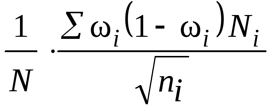
Более совершенной
формой отбора является пропорциональная
выборка. Пропорциональной называется
такая схема формирования выборочной
совокупности, когда численность выборок,
взятых из каждой типической группы в
генеральной совокупности, пропорциональна
численностям, дисперсиям (или комбинированно
и численностям, и дисперсиям). Условно
определяем численность выборки в 100
единиц и отбираем единицы из групп:
– пропорционально
численности их генеральной совокупности
(табл. 7.4). В таблице
обозначено:
Ni– численность типической группы;
dj
– доля (Ni/N);
N– численность
генеральной совокупности;
ni– численность выборки из типической
группы вычисляется:
![]() , (7.7)
, (7.7)
n – численность выборки из генеральной
совокупности.
Таблица
7.4
-
Группы
Ni
dj
ni
1
300
0,3
30
2
500
0,5
50
3
200
0,2
20
1000
1,0
100
–
пропорционально среднему квадратическому
отклонению(табл. 7.5).
здесь
i– среднее
квадратическое отклонение типических
групп;
ni
– численность выборки из типической
группы вычисляется по формуле

(7.8)
Таблица
7.5
-
Ni
i

ni
300
5
0,25
25
500
7
0,35
35
200
8
0,40
40
1000
20
1,0
100
–
комбинированно (табл. 7.6).
Численность
выборки вычисляется по формуле
![]() . (7.9)
. (7.9)
Таблица 7.6
-

i
iNi


300
5
1500
0,23
23
500
7
2100
0,53
53
200
8
1600
0.24
24
1000
20
6600
1,0
100
При проведении
типической выборки непосредственный
отбор из каждой группы проводится
методом случайного отбора.
Средние ошибки
выборки рассчитываются по формулам
табл. 7.7 в зависимости от способа отбора
из типических групп.
Таблица 7.7
|
Способ |
Повторный |
Бесповторный |
||
|
для |
для |
для |
для |
|
|
Непропорциональный |
|
|
|
|
|
Пропорциональный объему групп |
|
|
|
|
|
Пропорциональный |
|
|
|
|


здесь
![]() – средняя из внутригрупповых дисперсий
– средняя из внутригрупповых дисперсий
типических групп;
![]() – доля единиц, обладающих изучаемым
– доля единиц, обладающих изучаемым
признаком;
![]() – средняя из внутригрупповых дисперсий
– средняя из внутригрупповых дисперсий
для доли;
![]() – среднее квадратическое отклонение
– среднее квадратическое отклонение
в выборке изi-й типической группы;
![]() – объем выборки из типической группы;
– объем выборки из типической группы;
![]() – общий объем выборки;
– общий объем выборки;
![]() –
–
объем типической группы;
![]() – объем генеральной совокупности.
– объем генеральной совокупности.
Численность
выборки из каждой типической группы
должна быть пропорциональна среднему
квадратическому отклонению в этой
группе
![]() .Расчет численности
.Расчет численности
![]() производится по формулам, приведенным
производится по формулам, приведенным
в табл. 7.8.
Таблица 7.8
|
Повторный |
Бесповторный |
|
|
Для определения |
|
|
|
Для определения |
|
|


4. Серийная
выборка– удобена в тех случаях,
когда единицы совокупности объединены
в небольшие группы или серии. При серийной
выборке генеральную совокупность делят
на одинаковые по объему группы – серии.
В выборочную совокупность отбираются
серии. Сущность серийной выборки
заключается в случайном или механическом
отборе серий, внутри которых производится
сплошное обследование единиц. Средняя
ошибка серийной выборки с равновеликими
сериями зависит от величины только
межгрупповой дисперсии. Средние ошибки
сведены в табл. 7.9.
Таблица 7.9
|
Способ |
Формулы |
|
|
для |
для |
|
|
Повторный |
|
|
|
Бесповторный |
|
|


Здесь
R– число серий в генеральной
совокупности;
r – число
отобранных серий;
![]() – межсерийная (межгрупповая) дисперсия
– межсерийная (межгрупповая) дисперсия
средних;
![]() – межсерийная (межгрупповая) дисперсия
– межсерийная (межгрупповая) дисперсия
доли.
При серийном
отборе необходимую численность отбираемых
серий определяют так же, как и при
собственно-случайном методе отбора.
Расчет численности
серийной выборки производится по
формулам, приведенным в табл. 7.10.
Таблица 7.10
|
Повторный |
Бесповторный |
|
|
Для |
|
|
|
Для |
|
|


Пример.В
механическом цехе завода в десяти
бригадах работает 100 рабочих. В целях
изучения квалификации рабочих была
произведена 20 %-ная серийная бесповторная
выборка, в которую вошли две бригады.
Получено следующее распределение
обследованных рабочих по разрядам:
|
Рабочие |
Разряды рабочих |
Разряды рабочих |
Рабочие |
Разряды |
Разряды |
|
1 2 3 4 5 |
2 4 5 2 5 |
3 6 1 5 3 |
6 7 8 9 10 |
6 5 8 4 5 |
4 2 1 3 2 |
Необходимо
определить с вероятностью 0,997 пределы,
в которых находится средний разряд
рабочих механического цеха.
Решение.
Определим выборочные средние по
бригадам и общую среднюю как среднюю
взвешенную из групповых средних:

Определим
межсерийную дисперсию по формулам
(5.25):
![]()
Рассчитаем
среднюю ошибку выборки по формуле табл.
7.9:
![]()
Вычислим
предельную ошибку выборки с вероятностью
0,997:
![]()
С вероятностью
0,997 можно утверждать, что средний разряд
рабочих механического цеха находится
в пределах
![]()
Соседние файлы в предмете [НЕСОРТИРОВАННОЕ]
- #
- #
- #
- #
- #
- #
- #
- #
- #
- #
- #
From Wikipedia, the free encyclopedia
In statistics, the mean squared error (MSE)[1] or mean squared deviation (MSD) of an estimator (of a procedure for estimating an unobserved quantity) measures the average of the squares of the errors—that is, the average squared difference between the estimated values and the actual value. MSE is a risk function, corresponding to the expected value of the squared error loss.[2] The fact that MSE is almost always strictly positive (and not zero) is because of randomness or because the estimator does not account for information that could produce a more accurate estimate.[3] In machine learning, specifically empirical risk minimization, MSE may refer to the empirical risk (the average loss on an observed data set), as an estimate of the true MSE (the true risk: the average loss on the actual population distribution).
The MSE is a measure of the quality of an estimator. As it is derived from the square of Euclidean distance, it is always a positive value that decreases as the error approaches zero.
The MSE is the second moment (about the origin) of the error, and thus incorporates both the variance of the estimator (how widely spread the estimates are from one data sample to another) and its bias (how far off the average estimated value is from the true value).[citation needed] For an unbiased estimator, the MSE is the variance of the estimator. Like the variance, MSE has the same units of measurement as the square of the quantity being estimated. In an analogy to standard deviation, taking the square root of MSE yields the root-mean-square error or root-mean-square deviation (RMSE or RMSD), which has the same units as the quantity being estimated; for an unbiased estimator, the RMSE is the square root of the variance, known as the standard error.
Definition and basic properties[edit]
The MSE either assesses the quality of a predictor (i.e., a function mapping arbitrary inputs to a sample of values of some random variable), or of an estimator (i.e., a mathematical function mapping a sample of data to an estimate of a parameter of the population from which the data is sampled). The definition of an MSE differs according to whether one is describing a predictor or an estimator.
Predictor[edit]
If a vector of  predictions is generated from a sample of data points on all variables, and
  is the vector of observed values of the variable being predicted, with
  being the predicted values (e.g. as from a least-squares fit), then the within-sample MSE of the predictor is computed as

In other words, the MSE is the mean  of the squares of the errors
  . This is an easily computable quantity for a particular sample (and hence is sample-dependent).
In matrix notation,

where  is
is  and
and  is the
  column vector.
The MSE can also be computed on q data points that were not used in estimating the model, either because they were held back for this purpose, or because these data have been newly obtained. Within this process, known as statistical learning, the MSE is often called the test MSE,[4] and is computed as

Estimator[edit]
The MSE of an estimator  with respect to an unknown parameter
  is defined as[1]
![{displaystyle operatorname {MSE} ({hat {theta }})=operatorname {E} _{theta }left[({hat {theta }}-theta )^{2}right].}](https://wikimedia.org/api/rest_v1/media/math/render/svg/9a0e1b3bac58f9ba2d2f4ff8b85b2e35a8f4bf78)
This definition depends on the unknown parameter, but the MSE is a priori a property of an estimator. The MSE could be a function of unknown parameters, in which case any estimator of the MSE based on estimates of these parameters would be a function of the data (and thus a random variable). If the estimator is derived as a sample statistic and is used to estimate some population parameter, then the expectation is with respect to the sampling distribution of the sample statistic.
The MSE can be written as the sum of the variance of the estimator and the squared bias of the estimator, providing a useful way to calculate the MSE and implying that in the case of unbiased estimators, the MSE and variance are equivalent.[5]

Proof of variance and bias relationship[edit]
![{displaystyle {begin{aligned}operatorname {MSE} ({hat {theta }})&=operatorname {E} _{theta }left[({hat {theta }}-theta )^{2}right]\&=operatorname {E} _{theta }left[left({hat {theta }}-operatorname {E} _{theta }[{hat {theta }}]+operatorname {E} _{theta }[{hat {theta }}]-theta right)^{2}right]\&=operatorname {E} _{theta }left[left({hat {theta }}-operatorname {E} _{theta }[{hat {theta }}]right)^{2}+2left({hat {theta }}-operatorname {E} _{theta }[{hat {theta }}]right)left(operatorname {E} _{theta }[{hat {theta }}]-theta right)+left(operatorname {E} _{theta }[{hat {theta }}]-theta right)^{2}right]\&=operatorname {E} _{theta }left[left({hat {theta }}-operatorname {E} _{theta }[{hat {theta }}]right)^{2}right]+operatorname {E} _{theta }left[2left({hat {theta }}-operatorname {E} _{theta }[{hat {theta }}]right)left(operatorname {E} _{theta }[{hat {theta }}]-theta right)right]+operatorname {E} _{theta }left[left(operatorname {E} _{theta }[{hat {theta }}]-theta right)^{2}right]\&=operatorname {E} _{theta }left[left({hat {theta }}-operatorname {E} _{theta }[{hat {theta }}]right)^{2}right]+2left(operatorname {E} _{theta }[{hat {theta }}]-theta right)operatorname {E} _{theta }left[{hat {theta }}-operatorname {E} _{theta }[{hat {theta }}]right]+left(operatorname {E} _{theta }[{hat {theta }}]-theta right)^{2}&&operatorname {E} _{theta }[{hat {theta }}]-theta ={text{const.}}\&=operatorname {E} _{theta }left[left({hat {theta }}-operatorname {E} _{theta }[{hat {theta }}]right)^{2}right]+2left(operatorname {E} _{theta }[{hat {theta }}]-theta right)left(operatorname {E} _{theta }[{hat {theta }}]-operatorname {E} _{theta }[{hat {theta }}]right)+left(operatorname {E} _{theta }[{hat {theta }}]-theta right)^{2}&&operatorname {E} _{theta }[{hat {theta }}]={text{const.}}\&=operatorname {E} _{theta }left[left({hat {theta }}-operatorname {E} _{theta }[{hat {theta }}]right)^{2}right]+left(operatorname {E} _{theta }[{hat {theta }}]-theta right)^{2}\&=operatorname {Var} _{theta }({hat {theta }})+operatorname {Bias} _{theta }({hat {theta }},theta )^{2}end{aligned}}}](https://wikimedia.org/api/rest_v1/media/math/render/svg/2ac524a751828f971013e1297a33ca1cc4c38cd6)
An even shorter proof can be achieved using the well-known formula that for a random variable  ,
,  . By substituting with,
  , we have
![{displaystyle {begin{aligned}operatorname {MSE} ({hat {theta }})&=mathbb {E} [({hat {theta }}-theta )^{2}]\&=operatorname {Var} ({hat {theta }}-theta )+(mathbb {E} [{hat {theta }}-theta ])^{2}\&=operatorname {Var} ({hat {theta }})+operatorname {Bias} ^{2}({hat {theta }})end{aligned}}}](https://wikimedia.org/api/rest_v1/media/math/render/svg/864646cf4426e2b62a3caf9460382eec1a77fe4e)
But in real modeling case, MSE could be described as the addition of model variance, model bias, and irreducible uncertainty (see Bias–variance tradeoff). According to the relationship, the MSE of the estimators could be simply used for the efficiency comparison, which includes the information of estimator variance and bias. This is called MSE criterion.
In regression[edit]
In regression analysis, plotting is a more natural way to view the overall trend of the whole data. The mean of the distance from each point to the predicted regression model can be calculated, and shown as the mean squared error. The squaring is critical to reduce the complexity with negative signs. To minimize MSE, the model could be more accurate, which would mean the model is closer to actual data. One example of a linear regression using this method is the least squares method—which evaluates appropriateness of linear regression model to model bivariate dataset,[6] but whose limitation is related to known distribution of the data.
The term mean squared error is sometimes used to refer to the unbiased estimate of error variance: the residual sum of squares divided by the number of degrees of freedom. This definition for a known, computed quantity differs from the above definition for the computed MSE of a predictor, in that a different denominator is used. The denominator is the sample size reduced by the number of model parameters estimated from the same data, (n−p) for p regressors or (n−p−1) if an intercept is used (see errors and residuals in statistics for more details).[7] Although the MSE (as defined in this article) is not an unbiased estimator of the error variance, it is consistent, given the consistency of the predictor.
In regression analysis, «mean squared error», often referred to as mean squared prediction error or «out-of-sample mean squared error», can also refer to the mean value of the squared deviations of the predictions from the true values, over an out-of-sample test space, generated by a model estimated over a particular sample space. This also is a known, computed quantity, and it varies by sample and by out-of-sample test space.
Examples[edit]
Mean[edit]
Suppose we have a random sample of size from a population,  . Suppose the sample units were chosen with replacement. That is, the units are selected one at a time, and previously selected units are still eligible for selection for all draws. The usual estimator for the
  is the sample average

which has an expected value equal to the true mean (so it is unbiased) and a mean squared error of
![{displaystyle operatorname {MSE} left({overline {X}}right)=operatorname {E} left[left({overline {X}}-mu right)^{2}right]=left({frac {sigma }{sqrt {n}}}right)^{2}={frac {sigma ^{2}}{n}}}](https://wikimedia.org/api/rest_v1/media/math/render/svg/b4647a2cc4c8f9a4c90b628faad2dcf80c4aae84)
where  is the population variance.
For a Gaussian distribution, this is the best unbiased estimator (i.e., one with the lowest MSE among all unbiased estimators), but not, say, for a uniform distribution.
Variance[edit]
The usual estimator for the variance is the corrected sample variance:

This is unbiased (its expected value is ), hence also called the unbiased sample variance, and its MSE is[8]

where  is the fourth central moment of the distribution or population, and
  is the excess kurtosis.
However, one can use other estimators for which are proportional to  , and an appropriate choice can always give a lower mean squared error. If we define

then we calculate:
![{displaystyle {begin{aligned}operatorname {MSE} (S_{a}^{2})&=operatorname {E} left[left({frac {n-1}{a}}S_{n-1}^{2}-sigma ^{2}right)^{2}right]\&=operatorname {E} left[{frac {(n-1)^{2}}{a^{2}}}S_{n-1}^{4}-2left({frac {n-1}{a}}S_{n-1}^{2}right)sigma ^{2}+sigma ^{4}right]\&={frac {(n-1)^{2}}{a^{2}}}operatorname {E} left[S_{n-1}^{4}right]-2left({frac {n-1}{a}}right)operatorname {E} left[S_{n-1}^{2}right]sigma ^{2}+sigma ^{4}\&={frac {(n-1)^{2}}{a^{2}}}operatorname {E} left[S_{n-1}^{4}right]-2left({frac {n-1}{a}}right)sigma ^{4}+sigma ^{4}&&operatorname {E} left[S_{n-1}^{2}right]=sigma ^{2}\&={frac {(n-1)^{2}}{a^{2}}}left({frac {gamma _{2}}{n}}+{frac {n+1}{n-1}}right)sigma ^{4}-2left({frac {n-1}{a}}right)sigma ^{4}+sigma ^{4}&&operatorname {E} left[S_{n-1}^{4}right]=operatorname {MSE} (S_{n-1}^{2})+sigma ^{4}\&={frac {n-1}{na^{2}}}left((n-1)gamma _{2}+n^{2}+nright)sigma ^{4}-2left({frac {n-1}{a}}right)sigma ^{4}+sigma ^{4}end{aligned}}}](https://wikimedia.org/api/rest_v1/media/math/render/svg/cf22322412b8454c706d78671e5d94208675a6e0)
This is minimized when

For a Gaussian distribution, where  , this means that the MSE is minimized when dividing the sum by
  . The minimum excess kurtosis is
  ,[a] which is achieved by a Bernoulli distribution with p = 1/2 (a coin flip), and the MSE is minimized for
  Hence regardless of the kurtosis, we get a «better» estimate (in the sense of having a lower MSE) by scaling down the unbiased estimator a little bit; this is a simple example of a shrinkage estimator: one «shrinks» the estimator towards zero (scales down the unbiased estimator).
Further, while the corrected sample variance is the best unbiased estimator (minimum mean squared error among unbiased estimators) of variance for Gaussian distributions, if the distribution is not Gaussian, then even among unbiased estimators, the best unbiased estimator of the variance may not be 
Gaussian distribution[edit]
The following table gives several estimators of the true parameters of the population, μ and σ2, for the Gaussian case.[9]
| True value | Estimator | Mean squared error |
|---|---|---|
 |
= the unbiased estimator of the population mean,  |

|
 |
= the unbiased estimator of the population variance,  |

|
|
= the biased estimator of the population variance,  |

|
|
= the biased estimator of the population variance,  |

|
Interpretation[edit]
An MSE of zero, meaning that the estimator predicts observations of the parameter with perfect accuracy, is ideal (but typically not possible).
Values of MSE may be used for comparative purposes. Two or more statistical models may be compared using their MSEs—as a measure of how well they explain a given set of observations: An unbiased estimator (estimated from a statistical model) with the smallest variance among all unbiased estimators is the best unbiased estimator or MVUE (Minimum-Variance Unbiased Estimator).
Both analysis of variance and linear regression techniques estimate the MSE as part of the analysis and use the estimated MSE to determine the statistical significance of the factors or predictors under study. The goal of experimental design is to construct experiments in such a way that when the observations are analyzed, the MSE is close to zero relative to the magnitude of at least one of the estimated treatment effects.
In one-way analysis of variance, MSE can be calculated by the division of the sum of squared errors and the degree of freedom. Also, the f-value is the ratio of the mean squared treatment and the MSE.
MSE is also used in several stepwise regression techniques as part of the determination as to how many predictors from a candidate set to include in a model for a given set of observations.
Applications[edit]
- Minimizing MSE is a key criterion in selecting estimators: see minimum mean-square error. Among unbiased estimators, minimizing the MSE is equivalent to minimizing the variance, and the estimator that does this is the minimum variance unbiased estimator. However, a biased estimator may have lower MSE; see estimator bias.
- In statistical modelling the MSE can represent the difference between the actual observations and the observation values predicted by the model. In this context, it is used to determine the extent to which the model fits the data as well as whether removing some explanatory variables is possible without significantly harming the model’s predictive ability.
- In forecasting and prediction, the Brier score is a measure of forecast skill based on MSE.
Loss function[edit]
Squared error loss is one of the most widely used loss functions in statistics[citation needed], though its widespread use stems more from mathematical convenience than considerations of actual loss in applications. Carl Friedrich Gauss, who introduced the use of mean squared error, was aware of its arbitrariness and was in agreement with objections to it on these grounds.[3] The mathematical benefits of mean squared error are particularly evident in its use at analyzing the performance of linear regression, as it allows one to partition the variation in a dataset into variation explained by the model and variation explained by randomness.
Criticism[edit]
The use of mean squared error without question has been criticized by the decision theorist James Berger. Mean squared error is the negative of the expected value of one specific utility function, the quadratic utility function, which may not be the appropriate utility function to use under a given set of circumstances. There are, however, some scenarios where mean squared error can serve as a good approximation to a loss function occurring naturally in an application.[10]
Like variance, mean squared error has the disadvantage of heavily weighting outliers.[11] This is a result of the squaring of each term, which effectively weights large errors more heavily than small ones. This property, undesirable in many applications, has led researchers to use alternatives such as the mean absolute error, or those based on the median.
See also[edit]
- Bias–variance tradeoff
- Hodges’ estimator
- James–Stein estimator
- Mean percentage error
- Mean square quantization error
- Mean square weighted deviation
- Mean squared displacement
- Mean squared prediction error
- Minimum mean square error
- Minimum mean squared error estimator
- Overfitting
- Peak signal-to-noise ratio
Notes[edit]
- ^ This can be proved by Jensen’s inequality as follows. The fourth central moment is an upper bound for the square of variance, so that the least value for their ratio is one, therefore, the least value for the excess kurtosis is −2, achieved, for instance, by a Bernoulli with p=1/2.
References[edit]
- ^ a b «Mean Squared Error (MSE)». www.probabilitycourse.com. Retrieved 2020-09-12.
- ^ Bickel, Peter J.; Doksum, Kjell A. (2015). Mathematical Statistics: Basic Ideas and Selected Topics. Vol. I (Second ed.). p. 20.
If we use quadratic loss, our risk function is called the mean squared error (MSE) …
- ^ a b Lehmann, E. L.; Casella, George (1998). Theory of Point Estimation (2nd ed.). New York: Springer. ISBN 978-0-387-98502-2. MR 1639875.
- ^ Gareth, James; Witten, Daniela; Hastie, Trevor; Tibshirani, Rob (2021). An Introduction to Statistical Learning: with Applications in R. Springer. ISBN 978-1071614174.
- ^ Wackerly, Dennis; Mendenhall, William; Scheaffer, Richard L. (2008). Mathematical Statistics with Applications (7 ed.). Belmont, CA, USA: Thomson Higher Education. ISBN 978-0-495-38508-0.
- ^ A modern introduction to probability and statistics : understanding why and how. Dekking, Michel, 1946-. London: Springer. 2005. ISBN 978-1-85233-896-1. OCLC 262680588.
{{cite book}}: CS1 maint: others (link) - ^ Steel, R.G.D, and Torrie, J. H., Principles and Procedures of Statistics with Special Reference to the Biological Sciences., McGraw Hill, 1960, page 288.
- ^ Mood, A.; Graybill, F.; Boes, D. (1974). Introduction to the Theory of Statistics (3rd ed.). McGraw-Hill. p. 229.
- ^ DeGroot, Morris H. (1980). Probability and Statistics (2nd ed.). Addison-Wesley.
- ^ Berger, James O. (1985). «2.4.2 Certain Standard Loss Functions». Statistical Decision Theory and Bayesian Analysis (2nd ed.). New York: Springer-Verlag. p. 60. ISBN 978-0-387-96098-2. MR 0804611.
- ^ Bermejo, Sergio; Cabestany, Joan (2001). «Oriented principal component analysis for large margin classifiers». Neural Networks. 14 (10): 1447–1461. doi:10.1016/S0893-6080(01)00106-X. PMID 11771723.
1.1. Ошибки
выборочного наблюдения
Средняя
ошибка выборки показывает, как генеральная средняя отклоняется в среднем от выборочной средней в ту или другую сторону. Формула
расчета средней ошибки выборки определяется видом исследуемого признака единиц
совокупности (количественный или альтернативный) и
способом отбора (бесповторный или повторный).
·
Если отбор повторный, а признак количественный
средняя ошибка выборки определяется по формуле
![]() , где
, где ![]() — дисперсия признака в выборочной совокупности
— дисперсия признака в выборочной совокупности
n- число единиц
в выборке
·
Если отбор бесповторный, а признак
количественный
 , где N—
число единиц в генеральной совокупности
·
Если отбор повторный, а признак альтернативный
 , где w-выборочная
доля
·
Если отбор бесповторный, а признак
альтернативный

Предельная ошибка выборки— показывающая с определенной степенью вероятности
отклонения средней от выборочной средней.
Предельная ошибка выборки
![]() , где параметр t зависит
, где параметр t зависит
от вероятности
Некоторые значения параметра t приведены
в таблице:
|
Вероятность, p |
0.95 |
0.954 |
0.9876 |
0.9907 |
0.9973 |
0.9999 |
|
Параметр t |
1.96 |
2.0 |
2.5 |
2.6 |
3.0 |
4.0 |
·
Если отбор повторный, а признак количественный
средняя ошибка выборки определяется по формуле
![]() , где
, где ![]() — дисперсия признака в выборочной совокупности
— дисперсия признака в выборочной совокупности
n- число единиц
в выборке
·
Если отбор бесповторный, а признак
количественный
 , где N—
число единиц в генеральной совокупности
·
Если отбор повторный, а признак альтернативный
 , где w-выборочная
доля
·
Если отбор бесповторный, а признак
альтернативный

Доверительный интервал для генеральной средней
![]()
Доверительный интервал для
генеральной доли
![]()
Пример расчета доверительного
интервала:
При выборочном обследовании 5% продукции по методу случайного
бесповторного отбора получены данные о содержании сахара в образцах:
|
Сахарность, % |
Число |
|
16-17 17-18 18-19 19-20 20-21 |
10 158 154 50 28 |
|
На основании этих данных вычислите:
1. Средний процент сахаристости.
2. Дисперсию и среднее квадратическое
отклонение.
3. С вероятностью 0.954 возможные пределы среднего значения
сахаристости продукции для всей партии.
4. С вероятностью 0.997 возможный процент продукции высшего
сорта по всей партии, если известно, что из 400 проб, попавших в выборку , 80
ед. отнесены к продукции высшего сорта.
Решение.
1.
Средний процент сахаристости найдем по формуле средней взвешенной
![]() , где xi–
, где xi–
середина i-го интервала
![]() =18,32 %
=18,32 %
2.
Дисперсия
![]()
![]()
![]() =336,49
=336,49
D(X)=336.49–
18.322=0.8676
Среднее квадратическое отклонение
![]() =0,93%
=0,93%
5. Предельная ошибка для
среднего процента сахаристости
![]()
для вероятности 0,954 параметр t=2.0
![]()
Доверительный интервал для среднего значения процента
сахаристости
![]()
![]()
![]()
С вероятностью 0,954 можно утверждать, что в генеральной
совокупности средний процент сахаристости лежит в пределах от 18,23% до 18,41%.
5. Доля продукции высшего сорта в выборочной совокупности
![]()
Предельная ошибка для
доли продукции высшего сорта
![]()
для вероятности 0,997 параметр t=3.0
![]()
Доверительный интервал для доли продукции высшего сорта
![]()
![]()
![]()
С вероятностью 0,997 можно утверждать, что в генеральной
совокупности доля продукции высшего сорта лежит в пределах от 14,0% до 26,0%.
Теорема 1. Вероятность того, что
отклонение выборочной доли от генеральной
доли не превосходит числа
(по абсолютной величине), равна
![]()
, где
![]()
.
Последняя формула называется формулой
доверительной вероятности при оценке
доли признака.
Определение 1. Средней
квадратической ошибкой выборки при
оценке генеральной доли признака
называется среднее квадратическое
отклонение выборочной доли w
собственно-случайной выборки (для
бесповторной выборки обозначается
w).
Следствие 1. При заданной
доверительной вероятности
предельная ошибка выборки равна t-кратной
величине средней квадратической ошибки,
т.е.
![]()
.
Следствие 2. Доверительный
интервал для генеральной доли может
быть найден по формуле
![]()
.
Используя формулы дисперсий
и
![]()
при оценке генеральной доли признака
соответственно при повторной и
бесповторной собственно-случайной
выборке, можно получить формулы средних
квадратических ошибок:
|
|
|

Заметим, что генеральная доля p
неизвестна, но при достаточно большом
объеме выборки практически достоверно,
что pw.
Более того, если даже выборочная доля
w неизвестна, то в
качестве pq можно взять
его максимально возможное значение
0,25.
Теорема 2. Вероятность того, что
отклонение выборочной средней от
генеральной средней не превосходит
числа
(по абсолютной величине), равна
![]()
,
где
![]()
.
Последняя формула называется формулой
доверительной вероятности для средней.
Доказательство теоремы основано на
теореме Ляпунова и свойстве 2 случайной
величины, распределенной по нормальному
закону распределения.
Определение 2. Средней
квадратической ошибкой выборки при
оценке генеральной средней называется
среднее квадратическое отклонение
выборочной доли
![]()
собственно-случайной выборки (для
бесповторной выборки обозначается
![]()
).
Следствие 3. При заданной
доверительной вероятности
предельная ошибка выборки равна t-кратной
величине средней квадратической ошибки,
т.е.
![]()
.
Следствие 4. Доверительный
интервал для генеральной средней может
быть найден по формуле
![]()
.
Используя формулы дисперсий
и
![]()
при оценке генеральной средней
соответственно при повторной и
бесповторной собственно-случайной
выборке, можно получить формулы средних
квадратических ошибок:
|
|
|
Заметим, что дисперсия 2
неизвестна, но при достаточно большом
объеме выборки практически достоверно,
что s22.
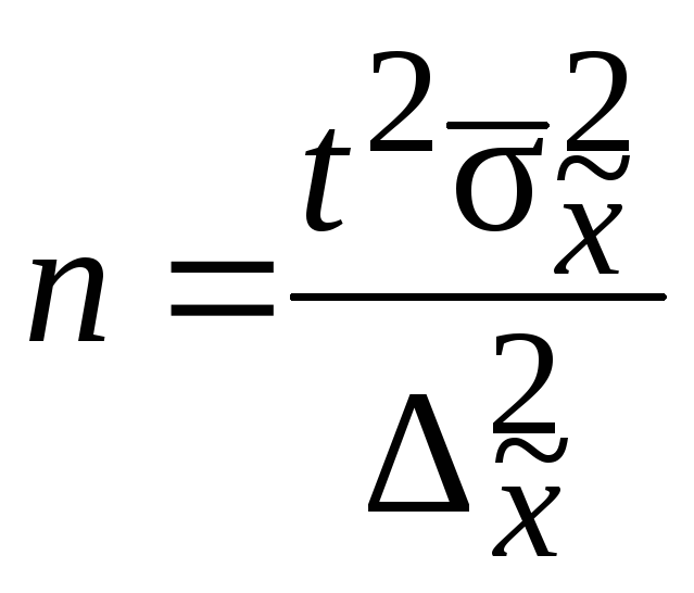
5. Определение необходимого объема повторной и бесповторной выборок
Для определения объема выборки n
необходимо знать надежность (доверительную
вероятность) оценки
и точность (предельную ошибку выборки)
.
Например, при оценке генеральной средней
для повторной выборки:
(t)=,
где
.
При заданной доверительной вероятности
предельная ошибка
выборки равна t-кратной
величине средней квадратической ошибки,
т.е.
(п.40, следствие 1).
Формула дисперсии
при оценке генеральной средней при
повторной собственно-случайной выборке
(п.36, теорема 1).
Следовательно,
![]()
.
Отсюда
![]()
.
Итак, для определения объема выборки
необходимо знать дисперсию генеральной
совокупности 2
, которая неизвестна. Обычно, с целью
определения 2
, проводят выборочное наблюдение (или
используют данные предыдущего аналогичного
исследования) и полагают, что s22.
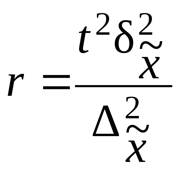
Аналогично находятся другие формулы
для определения объема выборки по
известным надежности и точности:
![]()
– при оценке генеральной средней для
бесповторной выборки;
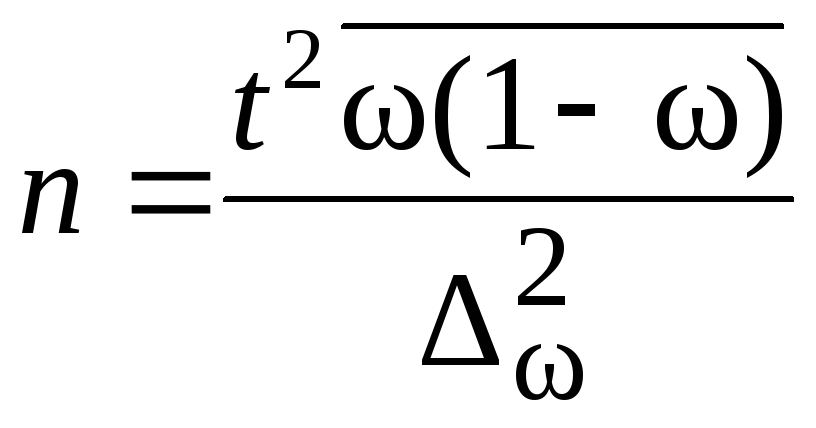
![]()
– при оценке генеральной доли для
повторной выборки;
![]()
– при оценке генеральной доли для
бесповторной выборки.
При оценке генеральной доли полагают
w
p.
Соседние файлы в предмете [НЕСОРТИРОВАННОЕ]
- #
- #
- #
- #
- #
- #
- #
- #
- #
- #
- #
From Wikipedia, the free encyclopedia
In statistics, the mean squared error (MSE)[1] or mean squared deviation (MSD) of an estimator (of a procedure for estimating an unobserved quantity) measures the average of the squares of the errors—that is, the average squared difference between the estimated values and the actual value. MSE is a risk function, corresponding to the expected value of the squared error loss.[2] The fact that MSE is almost always strictly positive (and not zero) is because of randomness or because the estimator does not account for information that could produce a more accurate estimate.[3] In machine learning, specifically empirical risk minimization, MSE may refer to the empirical risk (the average loss on an observed data set), as an estimate of the true MSE (the true risk: the average loss on the actual population distribution).
The MSE is a measure of the quality of an estimator. As it is derived from the square of Euclidean distance, it is always a positive value that decreases as the error approaches zero.
The MSE is the second moment (about the origin) of the error, and thus incorporates both the variance of the estimator (how widely spread the estimates are from one data sample to another) and its bias (how far off the average estimated value is from the true value).[citation needed] For an unbiased estimator, the MSE is the variance of the estimator. Like the variance, MSE has the same units of measurement as the square of the quantity being estimated. In an analogy to standard deviation, taking the square root of MSE yields the root-mean-square error or root-mean-square deviation (RMSE or RMSD), which has the same units as the quantity being estimated; for an unbiased estimator, the RMSE is the square root of the variance, known as the standard error.
Definition and basic properties[edit]
The MSE either assesses the quality of a predictor (i.e., a function mapping arbitrary inputs to a sample of values of some random variable), or of an estimator (i.e., a mathematical function mapping a sample of data to an estimate of a parameter of the population from which the data is sampled). The definition of an MSE differs according to whether one is describing a predictor or an estimator.
Predictor[edit]
If a vector of predictions is generated from a sample of data points on all variables, and is the vector of observed values of the variable being predicted, with being the predicted values (e.g. as from a least-squares fit), then the within-sample MSE of the predictor is computed as
In other words, the MSE is the mean of the squares of the errors . This is an easily computable quantity for a particular sample (and hence is sample-dependent).
In matrix notation,
where is and is the column vector.
The MSE can also be computed on q data points that were not used in estimating the model, either because they were held back for this purpose, or because these data have been newly obtained. Within this process, known as statistical learning, the MSE is often called the test MSE,[4] and is computed as
Estimator[edit]
The MSE of an estimator with respect to an unknown parameter is defined as[1]
This definition depends on the unknown parameter, but the MSE is a priori a property of an estimator. The MSE could be a function of unknown parameters, in which case any estimator of the MSE based on estimates of these parameters would be a function of the data (and thus a random variable). If the estimator is derived as a sample statistic and is used to estimate some population parameter, then the expectation is with respect to the sampling distribution of the sample statistic.
The MSE can be written as the sum of the variance of the estimator and the squared bias of the estimator, providing a useful way to calculate the MSE and implying that in the case of unbiased estimators, the MSE and variance are equivalent.[5]
Proof of variance and bias relationship[edit]
An even shorter proof can be achieved using the well-known formula that for a random variable , . By substituting with, , we have
But in real modeling case, MSE could be described as the addition of model variance, model bias, and irreducible uncertainty (see Bias–variance tradeoff). According to the relationship, the MSE of the estimators could be simply used for the efficiency comparison, which includes the information of estimator variance and bias. This is called MSE criterion.
In regression[edit]
In regression analysis, plotting is a more natural way to view the overall trend of the whole data. The mean of the distance from each point to the predicted regression model can be calculated, and shown as the mean squared error. The squaring is critical to reduce the complexity with negative signs. To minimize MSE, the model could be more accurate, which would mean the model is closer to actual data. One example of a linear regression using this method is the least squares method—which evaluates appropriateness of linear regression model to model bivariate dataset,[6] but whose limitation is related to known distribution of the data.
The term mean squared error is sometimes used to refer to the unbiased estimate of error variance: the residual sum of squares divided by the number of degrees of freedom. This definition for a known, computed quantity differs from the above definition for the computed MSE of a predictor, in that a different denominator is used. The denominator is the sample size reduced by the number of model parameters estimated from the same data, (n−p) for p regressors or (n−p−1) if an intercept is used (see errors and residuals in statistics for more details).[7] Although the MSE (as defined in this article) is not an unbiased estimator of the error variance, it is consistent, given the consistency of the predictor.
In regression analysis, «mean squared error», often referred to as mean squared prediction error or «out-of-sample mean squared error», can also refer to the mean value of the squared deviations of the predictions from the true values, over an out-of-sample test space, generated by a model estimated over a particular sample space. This also is a known, computed quantity, and it varies by sample and by out-of-sample test space.
Examples[edit]
Mean[edit]
Suppose we have a random sample of size from a population, . Suppose the sample units were chosen with replacement. That is, the units are selected one at a time, and previously selected units are still eligible for selection for all draws. The usual estimator for the is the sample average
which has an expected value equal to the true mean (so it is unbiased) and a mean squared error of
where is the population variance.
For a Gaussian distribution, this is the best unbiased estimator (i.e., one with the lowest MSE among all unbiased estimators), but not, say, for a uniform distribution.
Variance[edit]
The usual estimator for the variance is the corrected sample variance:
This is unbiased (its expected value is ), hence also called the unbiased sample variance, and its MSE is[8]
where is the fourth central moment of the distribution or population, and is the excess kurtosis.
However, one can use other estimators for which are proportional to , and an appropriate choice can always give a lower mean squared error. If we define
then we calculate:
This is minimized when
For a Gaussian distribution, where , this means that the MSE is minimized when dividing the sum by . The minimum excess kurtosis is ,[a] which is achieved by a Bernoulli distribution with p = 1/2 (a coin flip), and the MSE is minimized for Hence regardless of the kurtosis, we get a «better» estimate (in the sense of having a lower MSE) by scaling down the unbiased estimator a little bit; this is a simple example of a shrinkage estimator: one «shrinks» the estimator towards zero (scales down the unbiased estimator).
Further, while the corrected sample variance is the best unbiased estimator (minimum mean squared error among unbiased estimators) of variance for Gaussian distributions, if the distribution is not Gaussian, then even among unbiased estimators, the best unbiased estimator of the variance may not be
Gaussian distribution[edit]
The following table gives several estimators of the true parameters of the population, μ and σ2, for the Gaussian case.[9]
| True value | Estimator | Mean squared error |
|---|---|---|
|
= the unbiased estimator of the population mean, |
|
|
= the unbiased estimator of the population variance, |
|
|
= the biased estimator of the population variance, |
|
|
= the biased estimator of the population variance, |
|
Interpretation[edit]
An MSE of zero, meaning that the estimator predicts observations of the parameter with perfect accuracy, is ideal (but typically not possible).
Values of MSE may be used for comparative purposes. Two or more statistical models may be compared using their MSEs—as a measure of how well they explain a given set of observations: An unbiased estimator (estimated from a statistical model) with the smallest variance among all unbiased estimators is the best unbiased estimator or MVUE (Minimum-Variance Unbiased Estimator).
Both analysis of variance and linear regression techniques estimate the MSE as part of the analysis and use the estimated MSE to determine the statistical significance of the factors or predictors under study. The goal of experimental design is to construct experiments in such a way that when the observations are analyzed, the MSE is close to zero relative to the magnitude of at least one of the estimated treatment effects.
In one-way analysis of variance, MSE can be calculated by the division of the sum of squared errors and the degree of freedom. Also, the f-value is the ratio of the mean squared treatment and the MSE.
MSE is also used in several stepwise regression techniques as part of the determination as to how many predictors from a candidate set to include in a model for a given set of observations.
Applications[edit]
- Minimizing MSE is a key criterion in selecting estimators: see minimum mean-square error. Among unbiased estimators, minimizing the MSE is equivalent to minimizing the variance, and the estimator that does this is the minimum variance unbiased estimator. However, a biased estimator may have lower MSE; see estimator bias.
- In statistical modelling the MSE can represent the difference between the actual observations and the observation values predicted by the model. In this context, it is used to determine the extent to which the model fits the data as well as whether removing some explanatory variables is possible without significantly harming the model’s predictive ability.
- In forecasting and prediction, the Brier score is a measure of forecast skill based on MSE.
Loss function[edit]
Squared error loss is one of the most widely used loss functions in statistics[citation needed], though its widespread use stems more from mathematical convenience than considerations of actual loss in applications. Carl Friedrich Gauss, who introduced the use of mean squared error, was aware of its arbitrariness and was in agreement with objections to it on these grounds.[3] The mathematical benefits of mean squared error are particularly evident in its use at analyzing the performance of linear regression, as it allows one to partition the variation in a dataset into variation explained by the model and variation explained by randomness.
Criticism[edit]
The use of mean squared error without question has been criticized by the decision theorist James Berger. Mean squared error is the negative of the expected value of one specific utility function, the quadratic utility function, which may not be the appropriate utility function to use under a given set of circumstances. There are, however, some scenarios where mean squared error can serve as a good approximation to a loss function occurring naturally in an application.[10]
Like variance, mean squared error has the disadvantage of heavily weighting outliers.[11] This is a result of the squaring of each term, which effectively weights large errors more heavily than small ones. This property, undesirable in many applications, has led researchers to use alternatives such as the mean absolute error, or those based on the median.
See also[edit]
- Bias–variance tradeoff
- Hodges’ estimator
- James–Stein estimator
- Mean percentage error
- Mean square quantization error
- Mean square weighted deviation
- Mean squared displacement
- Mean squared prediction error
- Minimum mean square error
- Minimum mean squared error estimator
- Overfitting
- Peak signal-to-noise ratio
Notes[edit]
- ^ This can be proved by Jensen’s inequality as follows. The fourth central moment is an upper bound for the square of variance, so that the least value for their ratio is one, therefore, the least value for the excess kurtosis is −2, achieved, for instance, by a Bernoulli with p=1/2.
References[edit]
- ^ a b «Mean Squared Error (MSE)». www.probabilitycourse.com. Retrieved 2020-09-12.
- ^ Bickel, Peter J.; Doksum, Kjell A. (2015). Mathematical Statistics: Basic Ideas and Selected Topics. Vol. I (Second ed.). p. 20.
If we use quadratic loss, our risk function is called the mean squared error (MSE) …
- ^ a b Lehmann, E. L.; Casella, George (1998). Theory of Point Estimation (2nd ed.). New York: Springer. ISBN 978-0-387-98502-2. MR 1639875.
- ^ Gareth, James; Witten, Daniela; Hastie, Trevor; Tibshirani, Rob (2021). An Introduction to Statistical Learning: with Applications in R. Springer. ISBN 978-1071614174.
- ^ Wackerly, Dennis; Mendenhall, William; Scheaffer, Richard L. (2008). Mathematical Statistics with Applications (7 ed.). Belmont, CA, USA: Thomson Higher Education. ISBN 978-0-495-38508-0.
- ^ A modern introduction to probability and statistics : understanding why and how. Dekking, Michel, 1946-. London: Springer. 2005. ISBN 978-1-85233-896-1. OCLC 262680588.
{{cite book}}: CS1 maint: others (link) - ^ Steel, R.G.D, and Torrie, J. H., Principles and Procedures of Statistics with Special Reference to the Biological Sciences., McGraw Hill, 1960, page 288.
- ^ Mood, A.; Graybill, F.; Boes, D. (1974). Introduction to the Theory of Statistics (3rd ed.). McGraw-Hill. p. 229.
- ^ DeGroot, Morris H. (1980). Probability and Statistics (2nd ed.). Addison-Wesley.
- ^ Berger, James O. (1985). «2.4.2 Certain Standard Loss Functions». Statistical Decision Theory and Bayesian Analysis (2nd ed.). New York: Springer-Verlag. p. 60. ISBN 978-0-387-96098-2. MR 0804611.
- ^ Bermejo, Sergio; Cabestany, Joan (2001). «Oriented principal component analysis for large margin classifiers». Neural Networks. 14 (10): 1447–1461. doi:10.1016/S0893-6080(01)00106-X. PMID 11771723.
Средние ошибки повторной и бесповторной выборки
Средняя ошибка выборки
Средняя ошибка выборки представляет из себя такое расхождение между средними выборочной и генеральной совокупностями, которое не превышает ±б (дельта).
На основании теоремы Чебышева П. Л. величина средней ошибки при случайном повторном отборе в контрольных работах по статистике рассчитывается по формуле (для среднего количественного признака):

где числитель — дисперсия признака х в выборочной совокупности;
n — численность выборочной совокупности.
Для альтернативного признака формула средней ошибки выборки для доли по теореме Я. Бернулли рассчитывается по формуле:

где р(1- р) — дисперсия доли признака в генеральной совокупности;
n — объем выборки.
Вследствие, того что дисперсия признака в генеральной совокупности точно не известна, на практике используют значение дисперсии, которое рассчитано для выборочной совокупности на основании закона больших чисел. Согласно данному закону выборочная совокупность при большом объеме выборки достаточно точно воспроизводит характеристики генеральной совокупности.
Поэтому расчетные формулы средней ошибки при случайном повторном отборе будут выглядеть таким образом:
1. Для среднего количественного признака:

где S^2 — дисперсия признака х в выборочной совокупности;
n — объем выборки.
2. Для доли (альтернативного признака):

где w (1 — w) — дисперсия доли изучаемого признака в выборочной совокупности.
В теории вероятностей было показано, что генеральная дисперсия выражается через выборочную согласно формуле:

В случаях малой выборки, когда её объем меньше 30, необходимо учитывать коэффициент n/(n-1). Тогда среднюю ошибку малой выборки рассчитывают по формуле:

Так как в процессе бесповторной выборки сокращается численность единиц генеральной совокупности, то в представленных выше формулах расчета средних ошибок выборки нужно подкоренное выражение умножить на 1- (n/N).
Расчетные формулы для такого вида выборки будут выглядеть так:
1. Для средней количественного признака:

где N — объем генеральной совокупности; n — объем выборки.
2. Для доли (альтернативного признака):

где 1- (n/N) — доля единиц генеральной совокупности, не попавших в выборку.
Поскольку n всегда меньше N, то дополнительный множитель 1 — (n/N) всегда будет меньше единицы. Это означает, что средняя ошибка при бесповторном отборе всегда будет меньше, чем при повторном. Когда доля единиц генеральной совокупности, которые не попали в выборку, существенная, то величина 1 — (n/N) близка к единице и тогда расчет средней ошибки производится по общей формуле.
Средняя ошибка зависит от следующих факторов:
1. При выполнении принципа случайного отбора средняя ошибка выборки определяется во-первых объемом выборки: чем больше численность, тем меньше величины средней ошибки выборки. Генеральная совокупность характеризуется точнее тогда, когда больше единиц данной совокупности охватывает выборочное наблюдение
2. Средняя ошибка также зависит от степени варьирования признака. Степень варьирования характеризуется дисперсией. Чем меньше вариация признака (дисперсия), тем меньше средняя ошибка выборки. При нулевой дисперсии (признак не варьируется) средняя ошибка выборки равна нулю, таким образом, любая единица генеральной совокупности будет характеризовать всю совокупность по этому признаку.
Источник: Балинова B.C. Статистика в вопросах и ответах: Учеб. пособие. — М.: ТК. Велби, Изд-во Проспект, 2004. — 344 с.
11.2. Оценка результатов выборочного наблюдения
11.2.1. Средняя и предельная ошибки выборки. Построение доверительных границ для средней и доли
Средняя ошибка выборки показывает, насколько отклоняется в среднем параметр выборочной совокупности от соответствующего параметра генеральной. Если рассчитать среднюю из ошибок всех возможных выборок определенного вида заданного объема (n), извлеченных из одной и той же генеральной совокупности, то получим их обобщающую характеристику — среднюю ошибку выборки ( ).
).
В теории выборочного наблюдения выведены формулы для определения , которые индивидуальны для разных способов отбора (повторного и бесповторного), типов используемых выборок и видов оцениваемых статистических показателей.
Например, если применяется повторная собственно случайная выборка, то определяется как:
 — при оценивании среднего значения признака;
 — если признак альтернативный, и оценивается доля.
При бесповторном собственно случайном отборе в формулы вносится поправка (1 — n/N):
 — для среднего значения признака;
 — для доли.
Вероятность получения именно такой величины ошибки всегда равна 0,683. На практике же предпочитают получать данные с большей вероятностью, но это приводит к возрастанию величины ошибки выборки.
Предельная ошибка выборки ( ) равна t-кратному числу средних ошибок выборки (в теории выборки принято коэффициент t называть коэффициентом доверия):
 .
.
Если ошибку выборки увеличить в два раза (t = 2), то получим гораздо большую вероятность того, что она не превысит определенного предела (в нашем случае — двойной средней ошибки) — 0,954. Если взять t = 3, то доверительная вероятность составит 0,997 — практически достоверность.
Уровень предельной ошибки выборки зависит от следующих факторов:
- степени вариации единиц генеральной совокупности;
- объема выборки;
- выбранных схем отбора (бесповторный отбор дает меньшую величину ошибки);
- уровня доверительной вероятности.
Если объем выборки больше 30, то значение t определяется по таблице нормального распределения, если меньше — по таблице распределения Стьюдента.
Приведем некоторые значения коэффициента доверия из таблицы нормального распределения.
Таблица
11.2.
| Значение доверительной вероятности P | 0,683 | 0,954 | 0,997 |
|---|---|---|---|
| Значение коэффициента доверия t | 1,0 | 2,0 | 3,0 |
Доверительный интервал для среднего значения признака и для доли в генеральной совокупности устанавливается следующим образом:

Итак, определение границ генеральной средней и доли состоит из следующих этапов:
Ошибки выборки при различных видах отбора
- Собственно случайная и механическая выборка. Средняя ошибка собственно случайной и механической выборки находятся по формулам, представленным в табл. 11.3.
Таблица
11.3.
Формулы для расчета средней ошибки собственно случайной и механической выборки ()
 |
|
где |
Пример 11.2. Для изучения уровня фондоотдачи было проведено выборочное обследование 90 предприятий из 225 методом случайной повторной выборки, в результате которого получены данные, представленные в таблице.
Таблица
11.4.
| Уровень фондоотдачи, руб. | До 1,4 | 1,4-1,6 | 1,6-1,8 | 1,8-2,0 | 2,0-2,2 | 2,2 и выше | Итого |
|---|---|---|---|---|---|---|---|
| Количество предприятий | 13 | 15 | 17 | 15 | 16 | 14 | 90 |
В рассматриваемом примере имеем 40%-ную выборку (90 : 225 = 0,4, или 40%). Определим ее предельную ошибку и границы для среднего значения признака в генеральной совокупности по шагам алгоритма:
- По результатам выборочного обследования рассчитаем среднее значение и дисперсию в выборочной совокупности:
Таблица
11.5.
| Результаты наблюдения | Расчетные значения | |||
|---|---|---|---|---|
| уровень фондоотдачи, руб., xi | количество предприятий, fi | середина интервала, xixb4 | xixb4fi | xixb42fi |
| До 1,4 | 13 | 1,3 | 16,9 | 21,97 |
| 1,4-1,6 | 15 | 1,5 | 22,5 | 33,75 |
| 1,6-1,8 | 17 | 1,7 | 28,9 | 49,13 |
| 1,8-2,0 | 15 | 1,9 | 28,5 | 54,15 |
| 2,0-2,2 | 16 | 2,1 | 33,6 | 70,56 |
| 2,2 и выше | 14 | 2,3 | 32,2 | 74,06 |
| Итого | 90 | — | 162,6 | 303,62 |
Выборочная средняя
Выборочная дисперсия изучаемого признака

- Определяем среднюю ошибку повторной случайной выборки

- Зададим вероятность, на уровне которой будем говорить о величине предельной ошибки выборки. Чаще всего она принимается равной 0,999; 0,997; 0,954.

Для наших данных определим предельную ошибку выборки, например, с вероятностью 0,954. По таблице значений вероятности функции нормального распределения (см. выдержку из нее, приведенную в Приложении 1) находим величину коэффициента доверия t, соответствующего вероятности 0,954. При вероятности 0,954 коэффициент t равен 2.
- Предельная ошибка выборки с вероятностью 0,954 равна
- Найдем доверительные границы для среднего значения уровня фондоотдачи в генеральной совокупности


Таким образом, в 954 случаях из 1000 среднее значение фондоотдачи будет не выше 1,88 руб. и не ниже 1,74 руб.
Выше была использована повторная схема случайного отбора. Посмотрим, изменятся ли результаты обследования, если предположить, что отбор осуществлялся по схеме бесповторного отбора. В этом случае расчет средней ошибки проводится по формуле
Тогда при вероятности равной 0,954 величина предельной ошибки выборки составит:

Доверительные границы для среднего значения признака при бесповторном случайном отборе будут иметь следующие значения:

Сравнив результаты двух схем отбора, можно сделать вывод о том, что применение бесповторной случайной выборки дает более точные результаты по сравнению с применением повторного отбора при одной и той же доверительной вероятности. При этом, чем больше объем выборки, тем существеннее сужаются границы значений средней при переходе от одной схемы отбора к другой.
По данным примера определим, в каких границах находится доля предприятий с уровнем фондоотдачи, не превышающим значения 2,0 руб., в генеральной совокупности:
- рассчитаем выборочную долю.
Количество предприятий в выборке с уровнем фондоотдачи, не превышающим значения 2,0 руб., составляет 60 единиц. Тогда
m = 60, n = 90, w = m/n = 60 : 90 = 0,667;
- рассчитаем дисперсию доли в выборочной совокупности
 ;
;
- средняя ошибка выборки при использовании повторной схемы отбора составит

Если предположить, что была использована бесповторная схема отбора, то средняя ошибка выборки с учетом поправки на конечность совокупности составит

- зададим доверительную вероятность и определим предельную ошибку выборки.
При значении вероятности Р = 0,997 по таблице нормального распределения получаем значение для коэффициента доверия t = 3 (см. выдержку из нее, приведенную в Приложении 1):

- установим границы для генеральной доли с вероятностью 0,997:

Таким образом, с вероятностью 0,997 можно утверждать, что в генеральной совокупности доля предприятий с уровнем фондоотдачи, не превышающим значения 2,0 руб., не меньше, чем 54,7%, и не больше 78,7%.
- Типическая выборка. При типической выборке генеральная совокупность объектов разбита на k групп, тогда
N1 + N2 + … + Ni + … + Nk = N.
Объем извлекаемых из каждой типической группы единиц зависит от принятого способа отбора; их общее количество образует необходимый объем выборки
n1 + n2 + … + ni + … + nk = n.
Существуют следующие два способа организации отбора внутри типической группы: пропорциональной объему типических групп и пропорциональной степени колеблемости значений признака у единиц наблюдения в группах. Рассмотрим первый из них, как наиболее часто используемый.
Отбор, пропорциональный объему типических групп, предполагает, что в каждой из них будет отобрано следующее число единиц совокупности:
n = ni · Ni/N
где ni — количество извлекаемых единиц для выборки из i-й типической группы;
n — общий объем выборки;
Ni — количество единиц генеральной совокупности, составивших i-ю типическую группу;
N — общее количество единиц генеральной совокупности.
Отбор единиц внутри групп происходит в виде случайной или механической выборки.
Формулы для оценивания средней ошибки выборки для среднего и доли представлены в табл. 11.6.
Таблица
11.6.
Формулы для расчета средней ошибки выборки ( ) при использовании типического отбора, пропорционального объему типических групп
Здесь  — средняя из групповых дисперсий типических групп.
Пример 11.3. В одном из московских вузов проведено выборочное обследование студентов с целью определения показателя средней посещаемости вузовской библиотеки одним студентом за семестр. Для этого была использована 5%-ная бесповторная типическая выборка, типические группы которой соответствуют номеру курса. При отборе, пропорциональном объему типических групп, получены следующие данные:
Таблица
11.7.
| Номер курса | Всего студентов, чел., Ni | Обследовано в результате выборочного наблюдения, чел., ni | Среднее число посещений библиотеки одним студентом за семестр, xi | Внутригрупповая выборочная дисперсия,  |
|---|---|---|---|---|
| 1 | 650 | 33 | 11 | 6 |
| 2 | 610 | 31 | 8 | 15 |
| 3 | 580 | 29 | 5 | 18 |
| 4 | 360 | 18 | 6 | 24 |
| 5 | 350 | 17 | 10 | 12 |
| Итого | 2 550 | 128 | 8 | — |
Число студентов, которое необходимо обследовать на каждом курсе, рассчитаем следующим образом:
- общий объем выборочной совокупности:
n = 2550/130*5 =128 (чел.);
- количество единиц, отобранных из каждой типической группы:

аналогично для других групп:
n2 = 31 (чел.);
n3 = 29 (чел.);
n4 = 18 (чел.);
n5 = 17 (чел.).
Проведем необходимые расчеты.
- Выборочная средняя, исходя из значений средних типических групп, составит:
- Средняя из внутригрупповых дисперсий
- Средняя ошибка выборки:
С вероятностью 0,954 находим предельную ошибку выборки:
- Доверительные границы для среднего значения признака в генеральной совокупности:


Таким образом, с вероятностью 0,954 можно утверждать, что один студент за семестр посещает вузовскую библиотеку в среднем от семи до девяти раз.
- Малая выборка. В связи с небольшим объемом выборочной совокупности те формулы для определения ошибок выборки, которые использовались нами ранее при «больших» выборках, становятся неподходящими и требуют корректировки.
Среднюю ошибку малой выборки определяют по формуле

Предельная ошибка малой выборки:

Распределение значений выборочных средних всегда имеет нормальный закон распределения (или приближается к нему) при п > 100, независимо от характера распределения генеральной совокупности. Однако в случае малых выборок действует иной закон распределения — распределение Стьюдента. В этом случае коэффициент доверия находится по таблице t-распределения Стьюдента в зависимости от величины доверительной вероятности Р и объема выборки п. В Приложении 1 приводится фрагмент таблицы t-распределения Стьюдента, представленной в виде зависимости доверительной вероятности от объема выборки и коэффициента доверия t.
Пример 11.4. Предположим, что выборочное обследование восьми студентов академии показало, что на подготовку к контрольной работе по статистике они затратили следующее количество часов: 8,5; 8,0; 7,8; 9,0; 7,2; 6,2; 8,4; 6,6.
Оценим выборочные средние затраты времени и построим доверительный интервал для среднего значения признака в генеральной совокупности, приняв доверительную вероятность равной 0,95.
- Среднее значение признака в выборке равно
- Значение среднего квадратического отклонения составляет
- Средняя ошибка выборки:
- Значение коэффициента доверия t = 2,365 для п = 8 и Р = 0,95 .
- Предельная ошибка выборки:
- Доверительный интервал для среднего значения признака в генеральной совокупности:


То есть с вероятностью 0,95 можно утверждать, что затраты времени студента на подготовку к контрольной работе находятся в пределах от 6,9 до 8,5 ч.
11.2.2. Определение численности выборочной совокупности
Перед непосредственным проведением выборочного наблюдения всегда решается вопрос, сколько единиц исследуемой совокупности необходимо отобрать для обследования. Формулы для определения численности выборки выводят из формул предельных ошибок выборки в соответствии со следующими исходными положениями (табл. 11.7):
- вид предполагаемой выборки;
- способ отбора (повторный или бесповторный);
- выбор оцениваемого параметра (среднего значения признака или доли).
Кроме того, следует заранее определиться со значением доверительной вероятности, устраивающей потребителя информации, и с размером допустимой предельной ошибки выборки.
Таблица
11.8.
Формулы для определения численности выборочной совокупности

Примечание: при использовании приведенных в таблице формул рекомендуется получаемую численность выборки округлять в большую сторону для обеспечения некоторого запаса в точности.
Пример 11.5. Рассчитаем, сколько из 507 промышленных предприятий следует проверить налоговой инспекции, чтобы с вероятностью 0,997 определить долю предприятий с нарушениями в уплате налогов. По данным прошлого аналогичного обследования величина среднего квадратического отклонения составила 0,15; размер ошибки выборки предполагается получить не выше, чем 0,05.
При использовании повторного случайного отбора следует проверить
При бесповторном случайном отборе потребуется проверить

Как видим, использование бесповторного отбора позволяет проводить обследование гораздо меньшего числа объектов.
Пример 11.6. Планируется провести обследование заработной платы на предприятиях отрасли методом случайного бесповторного отбора. Какова должна быть численность выборочной совокупности, если на момент обследования в отрасли число занятых составляло 100 000 чел.? Предельная ошибка выборки не должна превышать 100 руб. с вероятностью 0,954. По результатам предыдущих обследований заработной платы в отрасли известно, что среднее квадратическое отклонение составляет 500 руб.

Следовательно, для решения поставленной задачи необходимо включить в выборку не менее 100 человек.
В статистика, то среднеквадратичная ошибка (MSE)[1][2] или среднеквадратическое отклонение (MSD) из оценщик (процедуры оценки ненаблюдаемой величины) измеряет средний квадратов ошибки — то есть средний квадрат разницы между оценочными и фактическими значениями. MSE — это функция риска, соответствующий ожидаемое значение квадрата ошибки потери. Тот факт, что MSE почти всегда строго положительный (а не нулевой), объясняется тем, что случайность или потому что оценщик не учитывает информацию это может дать более точную оценку.[3]
MSE — это мера качества оценки — она всегда неотрицательна, а значения, близкие к нулю, лучше.
МСЭ — второй момент (о происхождении) ошибки и, таким образом, включает в себя как отклонение оценщика (насколько разбросаны оценки от одного образец данных другому) и его предвзятость (насколько далеко среднее оценочное значение от истинного значения). Для объективный оценщик, MSE — это дисперсия оценки. Как и дисперсия, MSE имеет те же единицы измерения, что и квадрат оцениваемой величины. По аналогии с стандартное отклонение, извлечение квадратного корня из MSE дает среднеквадратичную ошибку или среднеквадратичное отклонение (RMSE или RMSD), который имеет те же единицы, что и оцениваемое количество; для несмещенной оценки RMSE — это квадратный корень из отклонение, известный как стандартная ошибка.
Определение и основные свойства
MSE либо оценивает качество предсказатель (т.е. функция, отображающая произвольные входные данные в выборку значений некоторых случайная переменная ) или оценщик (т.е. математическая функция отображение образец данных для оценки параметр из численность населения из которого берутся данные). Определение MSE различается в зависимости от того, описывается ли предсказатель или оценщик.
Предсказатель
Если вектор прогнозы генерируются из выборки п точки данных по всем переменным, и — вектор наблюдаемых значений прогнозируемой переменной, при этом будучи предсказанными значениями (например, по методу наименьших квадратов), то MSE в пределах выборки предсказателя вычисляется как

Другими словами, MSE — это иметь в виду  из квадраты ошибок
  . Это легко вычисляемая величина для конкретного образца (и, следовательно, зависит от образца).
В матрица обозначение
куда является и это матрица.
MSE также можно вычислить на q точки данных, которые не использовались при оценке модели, либо потому, что они были задержаны для этой цели, либо потому, что эти данные были получены заново. В этом процессе (известном как перекрестная проверка ), MSE часто называют среднеквадратичная ошибка прогноза, и вычисляется как

Оценщик
MSE оценщика по неизвестному параметру определяется как[2]
Это определение зависит от неизвестного параметра, но MSE априори свойство оценщика. MSE может быть функцией неизвестных параметров, и в этом случае любой оценщик MSE на основе оценок этих параметров будет функцией данных (и, следовательно, случайной величиной). Если оценщик выводится как статистика выборки и используется для оценки некоторого параметра совокупности, тогда ожидание относится к распределению выборки статистики выборки.
MSE можно записать как сумму отклонение оценщика и квадрата предвзятость оценщика, обеспечивая полезный способ вычисления MSE и подразумевая, что в случае несмещенных оценок MSE и дисперсия эквивалентны.[4]
Доказательство отношения дисперсии и предвзятости
- В качестве альтернативы у нас есть

Но в реальном случае моделирования MSE можно описать как добавление дисперсии модели, систематической ошибки модели и неснижаемой неопределенности. Согласно соотношению, MSE оценщиков может быть просто использована для эффективность сравнение, которое включает информацию о дисперсии и смещении оценки. Это называется критерием MSE.
В регрессе
В регрессивный анализ, построение графиков — более естественный способ просмотра общей тенденции всех данных. Среднее значение расстояния от каждой точки до прогнозируемой регрессионной модели может быть вычислено и показано как среднеквадратичная ошибка. Возведение в квадрат критически важно для уменьшения сложности с отрицательными знаками. Чтобы свести к минимуму MSE, модель может быть более точной, что означает, что модель ближе к фактическим данным. Одним из примеров линейной регрессии с использованием этого метода является метод наименьших квадратов —Который оценивает соответствие модели линейной регрессии модели двумерный набор данных[5], но чье ограничение связано с известным распределением данных.
Период, термин среднеквадратичная ошибка иногда используется для обозначения объективной оценки дисперсии ошибки: остаточная сумма квадратов делится на количество степени свободы. Это определение известной вычисленной величины отличается от приведенного выше определения вычисленной MSE предиктора тем, что используется другой знаменатель. Знаменатель — это размер выборки, уменьшенный на количество параметров модели, оцененных на основе тех же данных, (н-р) за п регрессоры или (п-п-1) если используется перехват (см. ошибки и остатки в статистике Больше подробностей).[6] Хотя MSE (как определено в этой статье) не является объективной оценкой дисперсии ошибки, она последовательный, учитывая непротиворечивость предсказателя.
В регрессионном анализе «среднеквадратичная ошибка», часто называемая среднеквадратичная ошибка прогноза или «среднеквадратичная ошибка вне выборки», также может относиться к среднему значению квадратичные отклонения прогнозов на основе истинных значений в тестовом пространстве вне выборки, сгенерированных моделью, оцененной в конкретном пространстве выборки. Это также известная вычисляемая величина, которая зависит от образца и тестового пространства вне образца.
Примеры
Иметь в виду
Предположим, у нас есть случайная выборка размера от населения, . Предположим, что образцы были выбраны с заменой. Это единицы выбираются по одному, и ранее выбранные единицы по-прежнему имеют право на выбор для всех рисует. Обычная оценка для это среднее по выборке[1]
ожидаемое значение которого равно истинному среднему значению (так что это беспристрастно) и среднеквадратичная ошибка
куда это дисперсия населения.
Для Гауссово распределение, это лучший объективный оценщик (то есть с самой низкой MSE среди всех несмещенных оценок), но не, скажем, для равномерное распределение.
Дисперсия
Обычной оценкой дисперсии является исправлено выборочная дисперсия:
Это объективно (его ожидаемое значение ), поэтому также называется объективная дисперсия выборки, и его MSE[7]
куда это четвертый центральный момент распределения или населения, и это избыточный эксцесс.
Однако можно использовать другие оценки для которые пропорциональны , и соответствующий выбор всегда может дать более низкую среднеквадратичную ошибку. Если мы определим
затем рассчитываем:
Это сводится к минимуму, когда
Для Гауссово распределение, куда , это означает, что MSE минимизируется при делении суммы на . Минимальный избыточный эксцесс составляет ,[а] что достигается за счет Распределение Бернулли с п = 1/2 (подбрасывание монеты), и MSE минимизируется для Следовательно, независимо от эксцесса, мы получаем «лучшую» оценку (в смысле наличия более низкой MSE), немного уменьшая несмещенную оценку; это простой пример оценщик усадки: один «сжимает» оценку до нуля (уменьшает несмещенную оценку).
Далее, хотя исправленная дисперсия выборки является лучший объективный оценщик (минимальная среднеквадратичная ошибка среди несмещенных оценок) дисперсии для гауссовских распределений, если распределение не является гауссовым, то даже среди несмещенных оценок лучшая несмещенная оценка дисперсии может не быть
Гауссово распределение
В следующей таблице приведены несколько оценок истинных параметров популяции, μ и σ.2, для гауссова случая.[8]
| Истинное значение | Оценщик | Среднеквадратичная ошибка |
|---|---|---|
|
= несмещенная оценка Средняя численность населения, |
|
|
= несмещенная оценка дисперсия населения, |
|
|
= смещенная оценка дисперсия населения, |
|
|
= смещенная оценка дисперсия населения, |
|
Интерпретация
MSE равна нулю, что означает, что оценщик предсказывает наблюдения параметра с идеальной точностью идеален (но обычно невозможен).
Значения MSE могут использоваться для сравнительных целей. Два и более статистические модели можно сравнить, используя их MSE — как меру того, насколько хорошо они объясняют данный набор наблюдений: несмещенная оценка (рассчитанная на основе статистической модели) с наименьшей дисперсией среди всех несмещенных оценок — это оценка лучший объективный оценщик или MVUE (несмещенная оценка минимальной дисперсии).
Обе линейная регрессия методы, такие как дисперсионный анализ оценить MSE как часть анализа и использовать оценочную MSE для определения Статистическая значимость изучаемых факторов или предикторов. Цель экспериментальная конструкция состоит в том, чтобы построить эксперименты таким образом, чтобы при анализе наблюдений MSE была близка к нулю относительно величины по крайней мере одного из оцененных эффектов лечения.
В односторонний дисперсионный анализ, MSE можно вычислить путем деления суммы квадратов ошибок и степени свободы. Кроме того, значение f — это отношение среднего квадрата обработки и MSE.
MSE также используется в нескольких пошаговая регрессия методы как часть определения того, сколько предикторов из набора кандидатов включить в модель для данного набора наблюдений.
Приложения
- Минимизация MSE является ключевым критерием при выборе оценщиков: см. минимальная среднеквадратичная ошибка. Среди несмещенных оценщиков минимизация MSE эквивалентна минимизации дисперсии, а оценщик, который делает это, является несмещенная оценка минимальной дисперсии. Однако смещенная оценка может иметь более низкую MSE; видеть систематическая ошибка оценки.
- В статистическое моделирование MSE может представлять разницу между фактическими наблюдениями и значениями наблюдений, предсказанными моделью. В этом контексте он используется для определения степени, в которой модель соответствует данным, а также возможности удаления некоторых объясняющих переменных без значительного ущерба для прогнозирующей способности модели.
- В прогнозирование и прогноз, то Оценка Бриера это мера умение прогнозировать на основе MSE.
Функция потерь
Квадратичная потеря ошибок — одна из наиболее широко используемых функции потерь в статистике[нужна цитата ], хотя его широкое использование проистекает больше из математического удобства, чем из соображений реальных потерь в приложениях. Карл Фридрих Гаусс, который ввел использование среднеквадратичной ошибки, сознавал ее произвол и был согласен с возражениями против нее на этих основаниях.[3] Математические преимущества среднеквадратичной ошибки особенно очевидны при ее использовании при анализе производительности линейная регрессия, поскольку он позволяет разделить вариацию в наборе данных на вариации, объясняемые моделью, и вариации, объясняемые случайностью.
Критика
Использование среднеквадратичной ошибки без вопросов подвергалось критике со стороны теоретик решений Джеймс Бергер. Среднеквадратичная ошибка — это отрицательное значение ожидаемого значения одного конкретного вспомогательная функция, квадратичная функция полезности, которая может не подходить для использования в данном наборе обстоятельств. Однако есть некоторые сценарии, в которых среднеквадратичная ошибка может служить хорошим приближением к функции потерь, естественным образом возникающей в приложении.[9]
подобно отклонение, среднеквадратичная ошибка имеет тот недостаток, что выбросы.[10] Это результат возведения в квадрат каждого члена, который фактически дает больший вес большим ошибкам, чем малым. Это свойство, нежелательное для многих приложений, заставило исследователей использовать альтернативы, такие как средняя абсолютная ошибка, или основанные на медиана.
Смотрите также
- Компромисс смещения и дисперсии
- Оценщик Ходжеса
- Оценка Джеймса – Стейна
- Средняя процентная ошибка
- Среднеквадратичная ошибка квантования
- Среднеквадратичное взвешенное отклонение
- Среднеквадратичное смещение
- Среднеквадратичная ошибка прогноза
- Минимальная среднеквадратичная ошибка
- Оценщик минимальной среднеквадратичной ошибки
- Пиковое отношение сигнал / шум
Примечания
- ^ Это может быть доказано Неравенство Дженсена следующим образом. Четвертый центральный момент является верхней границей квадрата дисперсии, так что наименьшее значение для их отношения равно единице, следовательно, наименьшее значение для избыточный эксцесс равно −2, что достигается, например, Бернулли с п=1/2.
Рекомендации
- ^ а б «Список вероятностных и статистических символов». Математическое хранилище. 2020-04-26. Получено 2020-09-12.
- ^ а б «Среднеквадратичная ошибка (MSE)». www.probabilitycourse.com. Получено 2020-09-12.
- ^ а б Lehmann, E. L .; Казелла, Джордж (1998). Теория точечного оценивания (2-е изд.). Нью-Йорк: Спрингер. ISBN 978-0-387-98502-2. Г-Н 1639875.
- ^ Вакерли, Деннис; Менденхолл, Уильям; Шеаффер, Ричард Л. (2008). Математическая статистика с приложениями (7-е изд.). Белмонт, Калифорния, США: Высшее образование Томсона. ISBN 978-0-495-38508-0.
- ^ Современное введение в вероятность и статистику: понимание, почему и как. Деккинг, Мишель, 1946-. Лондон: Спрингер. 2005 г. ISBN 978-1-85233-896-1. OCLC 262680588.CS1 maint: другие (ссылка на сайт)
- ^ Стил, Р.Г.Д., и Торри, Дж. Х., Принципы и процедуры статистики с особым акцентом на биологические науки., Макгроу Хилл, 1960, стр.288.
- ^ Настроение, А .; Graybill, F .; Боэс, Д. (1974). Введение в теорию статистики (3-е изд.). Макгроу-Хилл. п.229.
- ^ ДеГрут, Моррис Х. (1980). вероятность и статистика (2-е изд.). Эддисон-Уэсли.
- ^ Бергер, Джеймс О. (1985). «2.4.2 Некоторые стандартные функции потерь». Статистическая теория принятия решений и байесовский анализ (2-е изд.). Нью-Йорк: Springer-Verlag. п.60. ISBN 978-0-387-96098-2. Г-Н 0804611.
- ^ Бермехо, Серхио; Кабестани, Джоан (2001). «Ориентированный анализ главных компонентов для классификаторов с большой маржой». Нейронные сети. 14 (10): 1447–1461. Дои:10.1016 / S0893-6080 (01) 00106-X. PMID 11771723.
1.1. Ошибки
выборочного наблюдения
Средняя
ошибка выборки показывает, как генеральная средняя отклоняется в среднем от выборочной средней в ту или другую сторону. Формула
расчета средней ошибки выборки определяется видом исследуемого признака единиц
совокупности (количественный или альтернативный) и
способом отбора (бесповторный или повторный).
·
Если отбор повторный, а признак количественный
средняя ошибка выборки определяется по формуле
![]() , где
, где ![]() — дисперсия признака в выборочной совокупности
— дисперсия признака в выборочной совокупности
n- число единиц
в выборке
·
Если отбор бесповторный, а признак
количественный
, где N—
число единиц в генеральной совокупности
·
Если отбор повторный, а признак альтернативный
, где w-выборочная
доля
·
Если отбор бесповторный, а признак
альтернативный
Предельная ошибка выборки— показывающая с определенной степенью вероятности
отклонения средней от выборочной средней.
Предельная ошибка выборки
![]() , где параметр t зависит
, где параметр t зависит
от вероятности
Некоторые значения параметра t приведены
в таблице:
|
Вероятность, p |
0.95 |
0.954 |
0.9876 |
0.9907 |
0.9973 |
0.9999 |
|
Параметр t |
1.96 |
2.0 |
2.5 |
2.6 |
3.0 |
4.0 |
·
Если отбор повторный, а признак количественный
средняя ошибка выборки определяется по формуле
![]() , где
, где ![]() — дисперсия признака в выборочной совокупности
— дисперсия признака в выборочной совокупности
n- число единиц
в выборке
·
Если отбор бесповторный, а признак
количественный
, где N—
число единиц в генеральной совокупности
·
Если отбор повторный, а признак альтернативный
, где w-выборочная
доля
·
Если отбор бесповторный, а признак
альтернативный
Доверительный интервал для генеральной средней
![]()
Доверительный интервал для
генеральной доли
![]()
Пример расчета доверительного
интервала:
При выборочном обследовании 5% продукции по методу случайного
бесповторного отбора получены данные о содержании сахара в образцах:
|
Сахарность, % |
Число |
|
16-17 17-18 18-19 19-20 20-21 |
10 158 154 50 28 |
|
На основании этих данных вычислите:
1. Средний процент сахаристости.
2. Дисперсию и среднее квадратическое
отклонение.
3. С вероятностью 0.954 возможные пределы среднего значения
сахаристости продукции для всей партии.
4. С вероятностью 0.997 возможный процент продукции высшего
сорта по всей партии, если известно, что из 400 проб, попавших в выборку , 80
ед. отнесены к продукции высшего сорта.
Решение.
1.
Средний процент сахаристости найдем по формуле средней взвешенной
![]() , где xi–
, где xi–
середина i-го интервала
![]() =18,32 %
=18,32 %
2.
Дисперсия
![]()
![]()
![]() =336,49
=336,49
D(X)=336.49–
18.322=0.8676
Среднее квадратическое отклонение
![]() =0,93%
=0,93%
5. Предельная ошибка для
среднего процента сахаристости
![]()
для вероятности 0,954 параметр t=2.0
![]()
Доверительный интервал для среднего значения процента
сахаристости
![]()
![]()
![]()
С вероятностью 0,954 можно утверждать, что в генеральной
совокупности средний процент сахаристости лежит в пределах от 18,23% до 18,41%.
5. Доля продукции высшего сорта в выборочной совокупности
![]()
Предельная ошибка для
доли продукции высшего сорта
![]()
для вероятности 0,997 параметр t=3.0
![]()
Доверительный интервал для доли продукции высшего сорта
![]()
![]()
![]()
С вероятностью 0,997 можно утверждать, что в генеральной
совокупности доля продукции высшего сорта лежит в пределах от 14,0% до 26,0%.