
- sklearn.metrics.mean_squared_error(y_true, y_pred, *, sample_weight=None, multioutput=‘uniform_average’, squared=True)[source]
-
Mean squared error regression loss.
Read more in the User Guide.
- Parameters:
-
- y_truearray-like of shape (n_samples,) or (n_samples, n_outputs)
-
Ground truth (correct) target values.
- y_predarray-like of shape (n_samples,) or (n_samples, n_outputs)
-
Estimated target values.
- sample_weightarray-like of shape (n_samples,), default=None
-
Sample weights.
- multioutput{‘raw_values’, ‘uniform_average’} or array-like of shape (n_outputs,), default=’uniform_average’
-
Defines aggregating of multiple output values.
Array-like value defines weights used to average errors.- ‘raw_values’ :
-
Returns a full set of errors in case of multioutput input.
- ‘uniform_average’ :
-
Errors of all outputs are averaged with uniform weight.
- squaredbool, default=True
-
If True returns MSE value, if False returns RMSE value.
- Returns:
-
- lossfloat or ndarray of floats
-
A non-negative floating point value (the best value is 0.0), or an
array of floating point values, one for each individual target.
Examples
>>> from sklearn.metrics import mean_squared_error
>>> y_true = [3, -0.5, 2, 7]
>>> y_pred = [2.5, 0.0, 2, 8]
>>> mean_squared_error(y_true, y_pred)
0.375
>>> y_true = [3, -0.5, 2, 7]
>>> y_pred = [2.5, 0.0, 2, 8]
>>> mean_squared_error(y_true, y_pred, squared=False)
0.612...
>>> y_true = [[0.5, 1],[-1, 1],[7, -6]]
>>> y_pred = [[0, 2],[-1, 2],[8, -5]]
>>> mean_squared_error(y_true, y_pred)
0.708...
>>> mean_squared_error(y_true, y_pred, squared=False)
0.822...
>>> mean_squared_error(y_true, y_pred, multioutput='raw_values')
array([0.41666667, 1.        ])
>>> mean_squared_error(y_true, y_pred, multioutput=[0.3, 0.7])
0.825...
Examples using sklearn.metrics.mean_squared_error
Improve Article
Save Article
Like Article
Improve Article
Save Article
Like Article
The Mean Squared Error (MSE) or Mean Squared Deviation (MSD) of an estimator measures the average of error squares i.e. the average squared difference between the estimated values and true value. It is a risk function, corresponding to the expected value of the squared error loss. It is always non – negative and values close to zero are better. The MSE is the second moment of the error (about the origin) and thus incorporates both the variance of the estimator and its bias.
Steps to find the MSE
- Find the equation for the regression line.
(1)

- Insert X values in the equation found in step 1 in order to get the respective Y values i.e.
(2)

- Now subtract the new Y values (i.e. ) from the original Y values. Thus, found values are the error terms. It is also known as the vertical distance of the given point from the regression line.
(3)

- Square the errors found in step 3.
(4)

- Sum up all the squares.
(5)

- Divide the value found in step 5 by the total number of observations.
(6)


Example:
Consider the given data points: (1,1), (2,1), (3,2), (4,2), (5,4)
You can use this online calculator to find the regression equation / line.
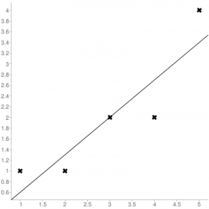
Regression line equation: Y = 0.7X – 0.1
| X | Y |  |
|---|---|---|
| 1 | 1 | 0.6 |
| 2 | 1 | 1.29 |
| 3 | 2 | 1.99 |
| 4 | 2 | 2.69 |
| 5 | 4 | 3.4 |
Now, using formula found for MSE in step 6 above, we can get MSE = 0.21606
MSE using scikit – learn:
from sklearn.metrics import mean_squared_error
Y_true = [1,1,2,2,4]
Y_pred = [0.6,1.29,1.99,2.69,3.4]
mean_squared_error(Y_true,Y_pred)
Output: 0.21606
MSE using Numpy module:
import numpy as np
Y_true = [1,1,2,2,4]
Y_pred = [0.6,1.29,1.99,2.69,3.4]
MSE = np.square(np.subtract(Y_true,Y_pred)).mean()
Output: 0.21606
Last Updated :
30 Jun, 2019
Like Article
Save Article
17 авг. 2022 г.
читать 1 мин
Среднеквадратическая ошибка (MSE) — это распространенный способ измерения точности предсказания модели. Он рассчитывается как:
MSE = (1/n) * Σ(фактическое – прогноз) 2
куда:
- Σ — причудливый символ, означающий «сумма».
- n – размер выборки
- фактический – фактическое значение данных
- прогноз – прогнозируемое значение данных
Чем ниже значение MSE, тем лучше модель способна точно предсказывать значения.
Как рассчитать MSE в Python
Мы можем создать простую функцию для вычисления MSE в Python:
import numpy as np

def mse(actual, pred):
 actual, pred = np.array(actual), np.array(pred)
 return np.square(np.subtract(actual,pred)).mean()
Затем мы можем использовать эту функцию для вычисления MSE для двух массивов: одного, содержащего фактические значения данных, и другого, содержащего прогнозируемые значения данных.
actual = [12, 13, 14, 15, 15, 22, 27]
pred = [11, 13, 14, 14, 15, 16, 18]

mse(actual, pred)

17.0
Среднеквадратическая ошибка (MSE) для этой модели оказывается равной 17,0 .
На практике среднеквадратическая ошибка (RMSE) чаще используется для оценки точности модели. Как следует из названия, это просто квадратный корень из среднеквадратичной ошибки.
Мы можем определить аналогичную функцию для вычисления RMSE:
import numpy as np

def rmse(actual, pred):
 actual, pred = np.array(actual), np.array(pred)
 return np.sqrt(np.square(np.subtract(actual,pred)).mean())
Затем мы можем использовать эту функцию для вычисления RMSE для двух массивов: одного, содержащего фактические значения данных, и другого, содержащего прогнозируемые значения данных.
actual = [12, 13, 14, 15, 15, 22, 27]
pred = [11, 13, 14, 14, 15, 16, 18]

rmse(actual, pred)

4.1231
Среднеквадратическая ошибка (RMSE) для этой модели оказывается равной 4,1231 .
Дополнительные ресурсы
Калькулятор среднеквадратичной ошибки (MSE)
Как рассчитать среднеквадратичную ошибку (MSE) в Excel
Время на прочтение
4 мин
Количество просмотров 3.7K

Функции потерь Python являются важной частью моделей машинного обучения. Эти функции показывают, насколько сильно предсказанный моделью результат отличается от фактического.
Существует несколько способов вычислить эту разницу. В этом материале мы рассмотрим некоторые из наиболее распространенных функций потерь.
Ниже будут рассмотрены следующие четыре функции потерь.
-
Среднеквадратическая ошибка
-
Среднеквадратическая ошибка
-
Средняя абсолютная ошибка
-
Кросс-энтропийные потери
Из этих четырех функций потерь первые три применяются к модели классификации.
1. Среднеквадратическая ошибка (MSE)
Среднеквадратичная ошибка (MSE) рассчитывается как среднее значение квадратов разностей между прогнозируемыми и фактически наблюдаемыми значениями. Математически это можно выразить следующим образом:
Реализация MSE на языке Python выглядит следующим образом:
import numpy as np # импортируем библиотеку numpy
def mean_squared_error(act, pred): # функция

   diff = pred - act # находим разницу между прогнозируемыми и наблюдаемыми значениями
   differences_squared = diff ** 2 # возводим в квадрат (чтобы избавиться от отрицательных значений)
   mean_diff = differences_squared.mean() # находим среднее значение

   return mean_diff

act = np.array([1.1,2,1.7]) # создаем список актуальных значений
pred = np.array([1,1.7,1.5]) # список прогнозируемых значений

print(mean_squared_error(act,pred))
Выход :
0.04666666666666667Вы также можете использовать mean_squared_error из sklearn для расчета MSE. Вот как работает функция:
from sklearn.metrics import mean_squared_error
act = np.array([1.1,2,1.7])
pred = np.array([1,1.7,1.5])
mean_squared_error(act, pred)
Выход :
0.04666666666666667
2. Корень среднеквадратической ошибки (RMSE)
Итак, ранее, для того, чтобы найти действительную ошибку среди между прогнозируемыми и фактически наблюдаемыми значениями (там могли быть положительные и отрицательные значения), мы возводили их в квадрат (для того чтобы отрицательные значения участвовали в расчетах в полной мере). Это была среднеквадратичная ошибка (MSE).
Корень среднеквадратической ошибки (RMSE) мы используем для того чтобы избавиться от квадратной степени, в которую мы ранее возвели действительную ошибку среди между прогнозируемыми и фактически наблюдаемыми значениями. Математически мы можем представить это следующим образом:
Реализация Python для RMSE выглядит следующим образом:
import numpy as np
def root_mean_squared_error(act, pred):

   diff = pred - act # находим разницу между прогнозируемыми и наблюдаемыми значениями
   differences_squared = diff ** 2 # возводим в квадрат
   mean_diff = differences_squared.mean() # находим среднее значение
   rmse_val = np.sqrt(mean_diff) # извлекаем квадратный корень
   return rmse_val

act = np.array([1.1,2,1.7])
pred = np.array([1,1.7,1.5])

print(root_mean_squared_error(act,pred))
Выход :
0.21602468994692867
Вы также можете использовать mean_squared_error из sklearn для расчета RMSE. Давайте посмотрим, как реализовать RMSE, используя ту же функцию:
from sklearn.metrics import mean_squared_error
act = np.array([1.1,2,1.7])
pred = np.array([1,1.7,1.5])
mean_squared_error(act, pred, squared = False) #Если установлено значение False, функция возвращает значение RMSE.
Выход :
0.21602468994692867
Если для параметра squared установлено значение True, функция возвращает значение MSE. Если установлено значение False, функция возвращает значение RMSE.
3. Средняя абсолютная ошибка (MAE)
Средняя абсолютная ошибка (MAE) рассчитывается как среднее значение абсолютной разницы между прогнозами и фактическими наблюдениями. Математически мы можем представить это следующим образом:
Реализация Python для MAE выглядит следующим образом:
import numpy as np
def mean_absolute_error(act, pred): #
    diff = pred - act # находим разницу между прогнозируемыми и наблюдаемыми значениями
    abs_diff = np.absolute(diff) # находим абсолютную разность между прогнозами и фактическими наблюдениями.
    mean_diff = abs_diff.mean() # находим среднее значение
    return mean_diff

act = np.array([1.1,2,1.7])
pred = np.array([1,1.7,1.5])
mean_absolute_error(act,pred)
Выход :
0.20000000000000004
Вы также можете использовать mean_absolute_error из sklearn для расчета MAE.
from sklearn.metrics import mean_absolute_error
act = np.array([1.1,2,1.7])
pred = np.array([1,1.7,1.5])
mean_absolute_error(act, pred)
Выход :
0.20000000000000004
4. Функция потерь перекрестной энтропии в Python
Функция потерь перекрестной энтропии также известна как отрицательная логарифмическая вероятность. Это чаще всего используется для задач классификации. Проблема классификации — это проблема, в которой вы классифицируете пример как принадлежащий к одному из более чем двух классов.
Давайте посмотрим, как вычислить ошибку в случае проблемы бинарной классификации.
Давайте рассмотрим проблему классификации, когда модель пытается провести классификацию между собакой и кошкой.
Код Python для поиска ошибки приведен ниже.
from sklearn.metrics import log_loss
log_loss(["Dog", "Cat", "Cat", "Dog"],[[.1, .9], [.9, .1], [.8, .2], [.35, .65]])
Выход :
0.21616187468057912
Мы используем метод log_loss из sklearn.
Первый аргумент в вызове функции — это список правильных меток классов для каждого входа. Второй аргумент — это список вероятностей, предсказанных моделью.
Вероятности представлены в следующем формате:
[P(dog), P(cat)]
Заключение
Это руководство было посвящено функциям потерь в Python. Мы рассмотрели различные функции потерь как для задач регрессии, так и для задач классификации. Надеюсь, вам понравился материал, ведь все было достаточно легко и понятно!
Кстати, для тех, кто хотел бы пойти дальше в изучении функций потерь, мы предлагаем разобрать одну вот такую — это очень интересная функция потерь Triplet Loss в Python (функцию тройных потерь), которую для вас любезно подготовил автор.
The mean squared error is a common way to measure the prediction accuracy of a model. In this tutorial, you’ll learn how to calculate the mean squared error in Python. You’ll start off by learning what the mean squared error represents. Then you’ll learn how to do this using Scikit-Learn (sklean), Numpy, as well as from scratch.
What is the Mean Squared Error
The mean squared error measures the average of the squares of the errors. What this means, is that it returns the average of the sums of the square of each difference between the estimated value and the true value.
The MSE is always positive, though it can be 0 if the predictions are completely accurate. It incorporates the variance of the estimator (how widely spread the estimates are) and its bias (how different the estimated values are from their true values).
The formula looks like below:

Now that you have an understanding of how to calculate the MSE, let’s take a look at how it can be calculated using Python.
Interpreting the Mean Squared Error
The mean squared error is always 0 or positive. When a MSE is larger, this is an indication that the linear regression model doesn’t accurately predict the model.
An important piece to note is that the MSE is sensitive to outliers. This is because it calculates the average of every data point’s error. Because of this, a larger error on outliers will amplify the MSE.
There is no “target” value for the MSE. The MSE can, however, be a good indicator of how well a model fits your data. It can also give you an indicator of choosing one model over another.
Loading a Sample Pandas DataFrame
Let’s start off by loading a sample Pandas DataFrame. If you want to follow along with this tutorial line-by-line, simply copy the code below and paste it into your favorite code editor.
# Importing a sample Pandas DataFrame
import pandas as pd

df = pd.DataFrame.from_dict({
    'x': [1,2,3,4,5,6,7,8,9,10],
    'y': [1,2,2,4,4,5,6,7,9,10]})

print(df.head())
#    x  y
# 0  1  1
# 1  2  2
# 2  3  2
# 3  4  4
# 4  5  4
You can see that the editor has loaded a DataFrame containing values for variables x and y. We can plot this data out, including the line of best fit using Seaborn’s .regplot() function:
# Plotting a line of best fit
import seaborn as sns
import matplotlib.pyplot as plt
sns.regplot(data=df, x='x', y='y', ci=None)
plt.ylim(bottom=0)
plt.xlim(left=0)
plt.show()
This returns the following visualization:
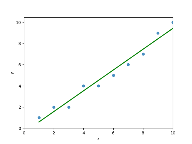
The mean squared error calculates the average of the sum of the squared differences between a data point and the line of best fit. By virtue of this, the lower a mean sqared error, the more better the line represents the relationship.
We can calculate this line of best using Scikit-Learn. You can learn about this in this in-depth tutorial on linear regression in sklearn. The code below predicts values for each x value using the linear model:
# Calculating prediction y values in sklearn
from sklearn.linear_model import LinearRegression

model = LinearRegression()
model.fit(df[['x']], df['y'])
y_2 = model.predict(df[['x']])
df['y_predicted'] = y_2
print(df.head())

# Returns:
#    x  y  y_predicted
# 0  1  1     0.581818
# 1  2  2     1.563636
# 2  3  2     2.545455
# 3  4  4     3.527273
# 4  5  4     4.509091
Calculating the Mean Squared Error with Scikit-Learn
The simplest way to calculate a mean squared error is to use Scikit-Learn (sklearn). The metrics module comes with a function, mean_squared_error() which allows you to pass in true and predicted values.
Let’s see how to calculate the MSE with sklearn:
# Calculating the MSE with sklearn
from sklearn.metrics import mean_squared_error
mse = mean_squared_error(df['y'], df['y_predicted'])
print(mse)

# Returns: 0.24727272727272714
This approach works very well when you’re already importing Scikit-Learn. That said, the function works easily on a Pandas DataFrame, as shown above.
In the next section, you’ll learn how to calculate the MSE with Numpy using a custom function.
Calculating the Mean Squared Error from Scratch using Numpy
Numpy itself doesn’t come with a function to calculate the mean squared error, but you can easily define a custom function to do this. We can make use of the subtract() function to subtract arrays element-wise.
# Definiting a custom function to calculate the MSE
import numpy as np

def mse(actual, predicted):
    actual = np.array(actual)
    predicted = np.array(predicted)
    differences = np.subtract(actual, predicted)
    squared_differences = np.square(differences)
    return squared_differences.mean()

print(mse(df['y'], df['y_predicted']))

# Returns: 0.24727272727272714
The code above is a bit verbose, but it shows how the function operates. We can cut down the code significantly, as shown below:
# A shorter version of the code above
import numpy as np

def mse(actual, predicted):
    return np.square(np.subtract(np.array(actual), np.array(predicted))).mean()

print(mse(df['y'], df['y_predicted']))

# Returns: 0.24727272727272714
Conclusion
In this tutorial, you learned what the mean squared error is and how it can be calculated using Python. First, you learned how to use Scikit-Learn’s mean_squared_error() function and then you built a custom function using Numpy.
The MSE is an important metric to use in evaluating the performance of your machine learning models. While Scikit-Learn abstracts the way in which the metric is calculated, understanding how it can be implemented from scratch can be a helpful tool.
Additional Resources
To learn more about related topics, check out the tutorials below:
- Pandas Variance: Calculating Variance of a Pandas Dataframe Column
- Calculate the Pearson Correlation Coefficient in Python
- How to Calculate a Z-Score in Python (4 Ways)
- Official Documentation from Scikit-Learn